FreeDiameter has been around for a while, and we’ve covered configuring the FreeDiameter components in Open5GS when it comes to the S6a interface, so you may have already come across FreeDiameter in the past, but been left a bit baffled as to how to get it to actually do something.
FreeDiameter is a FOSS implimentation of the Diameter protocol stack, and is predominantly used as a building point for developers to build Diameter applications on top of.
But for our scenario, we’ll just be using plain FreeDiameter.
So let’s get into it,
You’ll need FreeDiameter installed, and you’ll need a certificate for your FreeDiameter instance, more on that in this post.
Once that’s setup we’ll need to define some basics,
Inside freeDiameter.conf we’ll need to include the identity of our DRA, load the extensions and reference the certificate files:
The Wiki on the Sangoma documentation page is really out of date and can’t be easily edited by the public, so here’s the skinny on how to setup a Sangoma transcoding card on a modern Debian system:
apt-get install libxml2* wget make gcc
wget https://ftp.sangoma.com/linux/transcoding/sng-tc-linux-1.3.11.x86_64.tgz
tar xzf sng-tc-linux-1.3.11.x86_64.tgz
cd sng-tc-linux-1.3.11.x86_64/
make
make install
cp lib/* /usr/local/lib/
ldconfig
At this point you should be able to check for the presence of the card with:
sngtc_tool -dev ens33 -list_modules
Where ens33 is the name of the NIC that the server that shares a broadcast domain with the transcoder.
Successfully discovering the Sangoma D150 transcoder
If instead you see something like this:
root@fs-131:/etc/sngtc#  sngtc_tool -dev ens33 -list_modules
Failed to detect and initialize modules with size 1
That means the server can’t find the transcoding device. If you’re using a D150 (The Ethernet enabled versions) then you’ve got to make sure that the NIC you specified is on the same VLAN / broadcast domain as the server, for testing you can try directly connecting it to the NIC.
I also found I had to restart the device a few times to get it to a “happy” state.
It’s worth pointing out that there are no LEDs lit when the system is powered on, only when you connect a NIC.
Next we’ll need to setup the sngtc_server so these resources can be accessed via FreeSWITCH or Asterisk.
Config is pretty simple if you’re using an all-in-one deployment, all you’ll need to change is the NIC in a file you create in /etc/sngtc/sngtc_server.conf.xml:
<configuration name="sngtc_server.conf" description="Sangoma Transcoding Manager Configuration">

        <settings>
                <!--
                By default the SOAP server uses a private local IP and port that will work for out of the box installations
                where the SOAP client (Asterisk/FreeSWITCH) and server (sngtc_server) run in the same box.
                However, if you want to distribute multiple clients across the network, you need to edit this values to
                listen on an IP and port that is reachable for those clients.
                <param name="bindaddr" value="0.0.0.0" />
                <param name="bindport" value="9000" />
                -->
        </settings>

        <vocallos>

                <!-- The name of the vocallo is the ethernet device name as displayed by ifconfig -->
                <vocallo name="ens33">
                        <!-- Starting UDP port for the vocallo -->
                        <param name="base_udp" value="5000"/>
                        <!-- Starting IP address octet to use for the vocallo modules -->
                        <param name="base_ip_octet" value="182"/>
                </vocallo>

        </vocallos>


</configuration>
With that set we can actually try starting the server,
Again, all going well you should see something like this in the log:
Well, there’s another concept I haven’t introduced yet, and that’s ChargerS, this is a concept / component we’ll dig into deeper for derived charging, but for now just know we need to add a ChargerS rule in order to get CDRs rated:
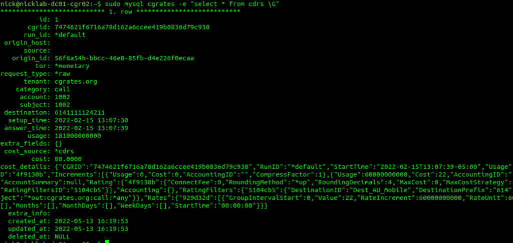
Well, if you’ve got CDR storage in StoreDB enabled (And you probably do if you’ve been following up until this point), then the answer is a MySQL table, and we can retrive the data with:
sudo mysql cgrates -e "select * from cdrs \G"
For those of you with a bit of MySQL experience under your belt, you’d be able to envisage using the SUM function to total a monthly bill for a customer from this.
Of course we can add CDRs via the API, and you probably already guessed this, but we can retrive CDRs via the API as well, filtering on the key criteria:
This would be useful for generating an invoice or populating recent calls for a customer portal.
Maybe creating rated CDRs and sticking them into a database is exactly what you’re looking to achieve in CGrateS – And if so, great, this is where you can stop – but for many use cases, there’s a want for an automated solution – For your platform to automatically integrate with CGrateS.
If you’ve got an Asterisk/FreeSWITCH/Kamailio or OpenSIPs based platform, then you can integrate CGrateS directly into your platform to add the CDRs automatically, as well as access features like prepaid credit control, concurrent call limits, etc, etc. The process is a little different on each of these platforms, but ultimately under the hood, all of these platforms have some middleware that generates the same API calls we just ran to create the CDR.
So far this tutorial has been heavy on teaching the API, because that’s what CGrateS ultimately is – An API service.
Our platforms like Asterisk and Kamailio with the CGrateS plugins are just CGrateS API clients, and so once we understand how to use and interact with the API it’s a breeze to plug in the module for your platform to generate the API calls to CGrateS required to integrate.
I build phone networks, and unfortunately, I’m not able to be everywhere at once.
This means sometimes I have to test things in networks I may not be within the coverage of.
To get around this, I’ve setup something pretty simple, but also pretty powerful – Remote test phones.
Using a Raspberry Pi, Intel NUC, or any old computer, I’m able to remotely control Android handsets out in the field, in the coverage footprint of whatever network I need.
This means I can make test calls, run speed testing, signal strength measurements, on real phones out in the network, without leaving my office.
Base OS
Because of some particularities with Wayland and X11, for this I’d steer clear of Ubuntu distributions, and suggest using Debian if you’re using x86 hardware, and Raspbian if you’re using a Pi.
Setup Android Debug Bridge (adb)
The base of this whole system is ADB, the Android Debug Bridge, which exposes the ability to remotely control an Android phone over USB.
You can also do this over WiFi, but I find for device testing, wired allows me to airplane mode a device or disable data, which I can’t do if the device is connected to ADB via WiFi.
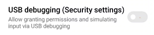
There’s lot of info online about setting Android Debug Bridge up on your device, unlocking the Developer Mode settings, etc, if you’ve not done this before I’ll just refer you to the official docs.
Before we plug in the phones we’ll need to setup the software on our remote testing machine, which is simple enough:
Now we can plug in each of the remote phones we want to use for testing and run the command “adb devices” which should list the phones with connected to the machine with ADB enabled:
[email protected]:~$ adb devices
List of devices attached
ABCDEFGHIJK	unauthenticated
LMNOPQRSTUV	unauthenticated
You’ll get a popup on each device asking if you want to allow USB debugging – If this is going to be a set-and-forget deployment, make sure you tick “Always allow from this Computer” so you don’t have to drive out and repeat this step, and away you go.
Lastly we can run adb devices again to confirm everything is in the connected state
Scrcpy
scrcpy an open-source remote screen mirror / controller that allows us to control Android devices from a computer.
In our case we’re going to install with Snap (if you hate snaps as many folks do, you can also compile from source):
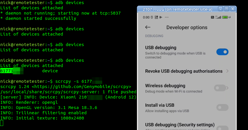
After SSHing into the box, we can just run scrcpy and boom, there’s the window we can interact with.
If you’ve got multiple devices connected to the same device, you’ll need to specify the ADB device ID, and of course, you can have multiple sessions open at the same time.
scrcpy -s 61771fe5
That’s it, as simple as that.
Tweaking
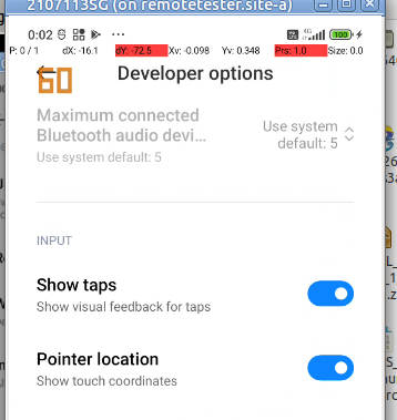
A few settings you may need to set:
I like to enable the “Show taps” option so I can see where my mouse is on the touchscreen and see what I’ve done, it makes it a lot easier when recording from the screen as well for the person watching to follow along.
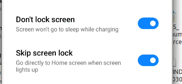
You’ll probably also want to disable the lock screen and keep the screen awake
Some OEMs have an additonal tick box if you want to be able to interact with the device (rather than just view the screen), which often requires signing into an account, if you see this toggle, you’ll need to turn it on:
Ansible Playbook
I’ve had to build a few of these, so I’ve put an Ansible Playbook on Github so you can create your own.
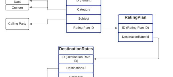
In our last post we introduced the CGrateS API and we used it to add Rates, Destinations and define DestinationRates.
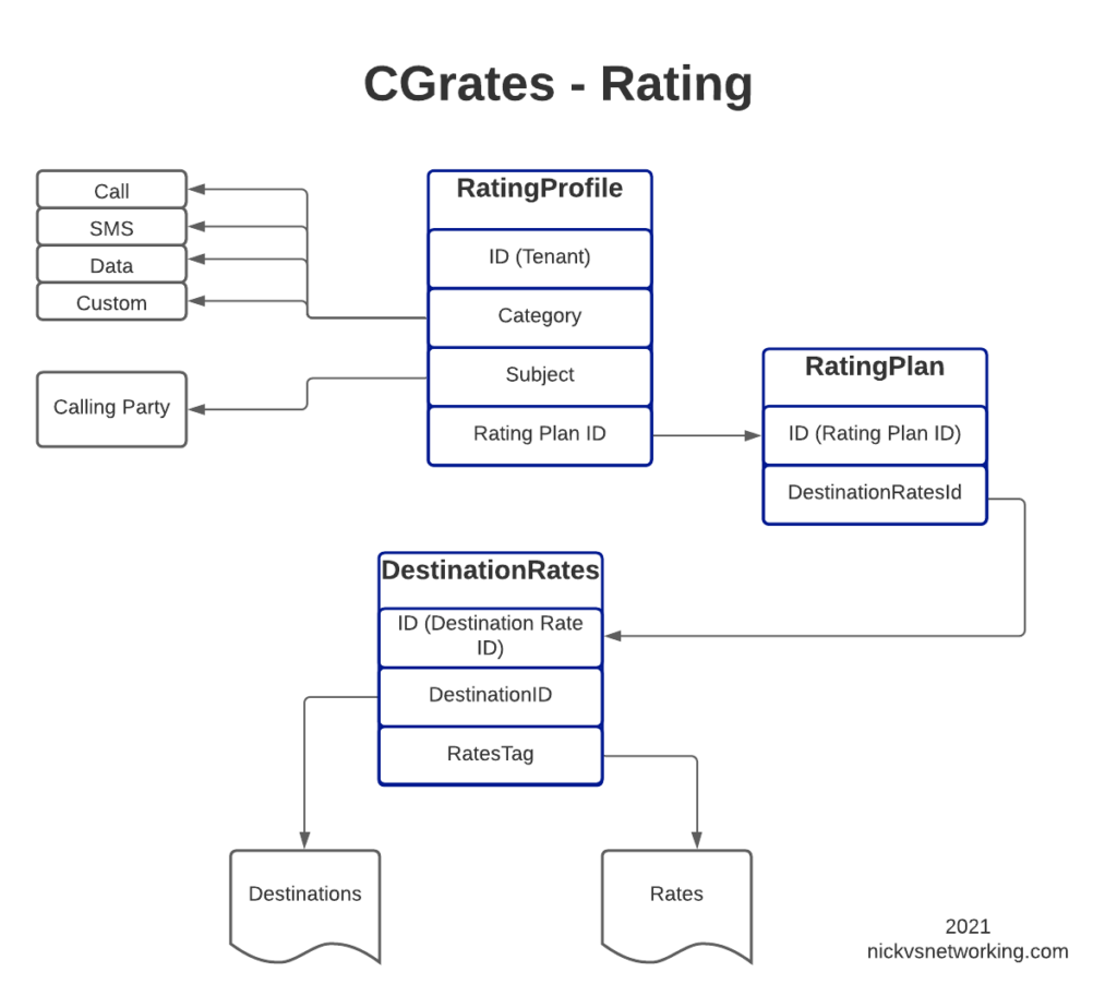
In this post, we’ll create the RatingPlan that references the DestinationRate we just defined, and the RatingProfile that references the RatingPlan, and then, as the cherry on top – We’ll rate some calls.
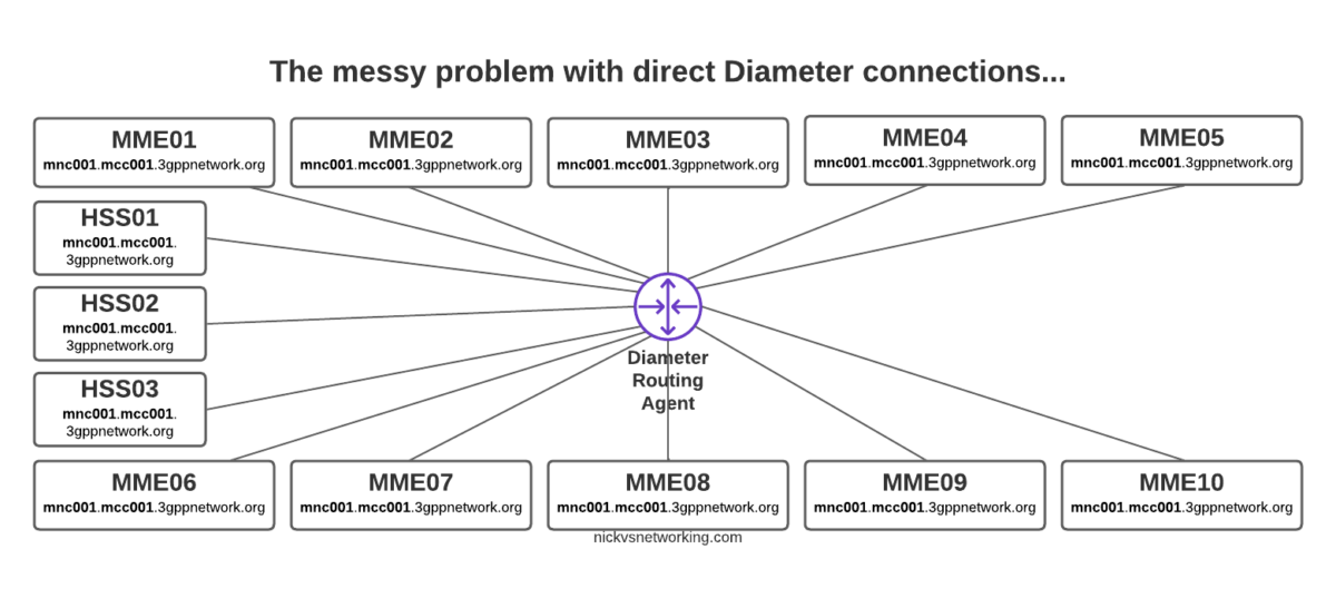
For anyone looking at the above diagram for the first time, you might be inclined to ask why what is the purpose of having all these layers?
This layered architecture allows all sorts of flexibility, that we wouldn’t otherwise have, for example, we can have multiple RatingPlans defined for the same Destinations, to allow us to have different Products defined, with different destinations and costs.
Likewise we can have multiple RatingProfiles assigned for the same destinations to allow us to generate multiple CDRs for each call, for example a CDR to bill the customer with and a CDR with our wholesale cost.
All this flexibility is enabled by the layered architecture.
Define RatingPlan
Picking up where we left off having just defined the DestinationRate, we’ll need to create a RatingPlan and link it to the DestinationRate, so let’s check on our DestinationRates:
From the output we can see we’ve got the DestinationRate defined, there’s a lot of info returned (I’ve left out most of it), but you can see the Destination, and the Rate associated with it is returned:
So after confirming that our DestinationRates are there, we’ll create a RatingPlan to reference it, for this we’ll use the APIerSv1.SetTPRatingPlan API call.
In our basic example, this really just glues the DestinationRate_AU object to RatingPlan_VoiceCalls.
It’s worth noting that you can use a RatingPlan to link to multiple DestinationRates, for example, we might want to have a different RatingPlan for each region / country, we can do that pretty easily too, in the below example I’ve referenced other Destination Rates (You’d go about defining the DestinationRates for these other destinations / rates the same way as we did in the last example).
One last step before we can test this all end-to-end, and that’s to link the RatingPlan we just defined with a RatingProfile.
StorDB & DataDB
Psych! Before we do that, I’m going to subject you to learning about backends for a while.
So far we’ve skirted around CGrateS architecture, but this is something we need to know for now.
To keep everything fast, a lot of data is cached in what is called a DataDB (if you’ve followed since part 1, then your DataDB is Redis, but there are other options).
To keep everything together, databases are used for storage, called StorDB (in our case we are using MySQL, but again, we can have other options) but calls to this database are minimal to keep the system fast.
If you’re an astute reader, you may have noticed many of our API calls have TP in method name, if the API call has TP in the name, it is storing it in the StoreDB, if it doesn’t, it means it’s storing it only in DataDB.
Why does this matter? Well, let’s look a little more closely and it will become clear:
ApierV1.SetRatingProfile will set the data only in DataDB (Redis), because it’s in the DataDB the change will take effect immediately.
ApierV1.SetTPRatingProfile will set the data only in StoreDB (MySQL), it will not take effect until it is copied from the database (StoreDB) to the cache (DataDB).
After we define the RatingPlan, we need to run this command prior to creating the RatingProfile, so it has something to reference, so we’ll do that by adding:
The last piece of the puzzle to define is the RatingProfile.
We define a few key things in the rating profile:
The Tenant – CGrateS is multitenant out of the box (in our case we’ve used tenant named “cgrates.org“, but you could have different tenants for different customers).
The Category – As we covered in the first post, CGrateS can bill voice calls, SMS, MMS & Data consumption, in this scenario we’re billing calls so we have the value set to *call, but we’ve got many other options. We can use Category to link what RatingPlan is used, for example we might want to offer a premium voice service with guaranteed CLI rates, using a different RatingPlan that charges more per call, or maybe we’re doing mobile and we want a different RatingPlan for use when Roaming, we can use Category to switch that.
The Subject – This is loosely the Source / Calling Party; in our case we’re using a wildcard value *any which will match any Subject
The RatingPlanActivations list the RatingPlanIds of the RatingPlans this RatingProfile uses
So let’s take a look at what we’d run to add this:
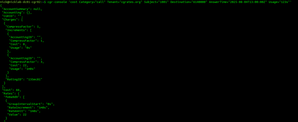
Okay, so at this point, all going well, we should have some data loaded, we’ve gone through all those steps to load this data, so now let’s simulate a call to a Mobile Number (22c per minute) for 123 seconds.
We cheated a fair bit, to show something that worked, but it’s not something you’d probably want to use in real life, loading static CSV files gets us off the ground, but in reality we don’t want to manage a system through CSV files.
Instead, we’d want to use an API.
Fair warning – There is some familiarity expected with JSON and RESTful APIs required, we’ll use Python3 for our examples, but you can use any programing language you’re comfortable with, or even CURL commands.
So we’re going to start by clearing out all the data we setup in CGrateS using the cgr-loader tool from those imported CSVs:
redis-cli flushall
sudo mysql -Nse 'show tables' cgrates | while read table; do sudo mysql -e "truncate table $table" cgrates; done
cgr-migrator -exec=*set_versions -stordb_passwd=CGRateS.org
sudo systemctl restart cgrates
So what have we just done? Well, we’ve just cleared all the data in CGrateS. We’re starting with a blank slate.
In this post, we’re going to define some Destinations, some Rates to charge and then some DestinationRates to link each Destination to a Rate.
But this time we’ll be doing this through the CGrateS API.
Introduction to the CGrateS API
CGrateS is all API driven – so let’s get acquainted with this API.
I’ve written a simple Python wrapper you can find here that will make talking to CGRateS a little easier, so let’s take it for a spin and get the Destinations that are loaded into our system:
import cgrateshttpapi
CGRateS_Obj = cgrateshttpapi.CGRateS('172.16.41.133', 2080) #Replace this IP with the IP Address of your CGrateS instance...

destinations = CGRateS_Obj.SendData({'method':'ApierV1.GetTPDestinationIDs','params':[{"TPid":"cgrates.org"}]})['result']

#Pretty print the result:
print("Destinations: ")
pprint.pprint(destinations)
All going well you’ll see something like this back:
Initializing with host 172.16.41.133 on port 2080
Sending Request with Body:
{'method': 'ApierV2.Ping', 'params': [{'Tenant': 'cgrates.org'}]}
Sending Request with Body:
{'method': 'ApierV2.GetTPDestinationIDs', 'params': [{"TPid":"cgrates.org"}]}
Destinations from CGRates: []
So what did we just do? Well, we sent a JSON formatted string to the CGRateS API at 172.16.41.133 on port 2080 – You’ll obviously need to change this to the IP of your CGrateS instance.
In the JSON body we sent we asked for all the Destinations using the ApierV1.GetTPDestinationIDs method, for the TPid ‘cgrates.org’,
And it looks like no destinations were sent back, so let’s change that!
Note: There’s API Version 1 and API Version 2, not all functions exist in both (at least not in the docs) so you have to use a mix.
Adding Destinations via the API
So now we’ve got our API setup, let’s see if we can add a destination!
To add a destination, we’ll need to go to the API guide and find the API call to add a destination – in our case the API call is ApierV2.SetTPDestination and will look like this:
So we’re creating a Destination named Dest_AU_Mobile and Prefix 614 will match this destination.
Note: I like to prefix all my Destinations with Dest_, all my rates with Rate_, etc, so it makes it easy when reading what’s going on what object is what, you may wish to do the same!
So we’ll use the Python code we had before to list the destinations, but this time, we’ll use the ApierV2.SetTPDestination API call to add a destination before listing them, let’s take a look:
If we post this to the CGR engine, we’ll create a rate, named Rate_AU_Mobile_Rate_1 that bills 22 cents per minute, charged every 60 seconds.
Let’s add a few rates:
CGRateS_Obj.SendData({"method":"ApierV1.SetTPRate","params":[{"ID":"Rate_AU_Mobile_Rate_1","TPid":"cgrates.org","RateSlots":[{"ConnectFee":0,"Rate":22,"RateUnit":"60s","RateIncrement":"60s","GroupIntervalStart":"0s"}]}],"id":1})
CGRateS_Obj.SendData({"method":"ApierV1.SetTPRate","params":[{"ID":"Rate_AU_Fixed_Rate_1","TPid":"cgrates.org","RateSlots":[{"ConnectFee":0,"Rate":14,"RateUnit":"60s","RateIncrement":"60s","GroupIntervalStart":"0s"}]}],"id":1})
CGRateS_Obj.SendData({"method":"ApierV1.SetTPRate","params":[{"ID":"Rate_AU_Toll_Free_Rate_1","TPid":"cgrates.org","RateSlots":[{"ConnectFee":25,"Rate":0,"RateUnit":"60s","RateIncrement":"60s","GroupIntervalStart":"0s"}]}],"id":1})

TPRateIds = CGRateS_Obj.SendData({"method":"ApierV1.GetTPRateIds","params":[{"TPid":"cgrates.org"}]})['result']
print(TPRateIds)
for TPRateId in TPRateIds:
    print("\tRate: " + str(TPRateId))
All going well, when you add the above, we’ll have added 3 new rates:
Rate Name
Cost
Rate_AU_Fixed_Rate_1
14c per minute charged every 60s
Rate_AU_Mobile_Rate_1
22c per minute charged every 60s
Rate_AU_Toll_Free_Rate_1
25c connection, untimed
Rates we just created
Linking Rates to Destinations
So now with Destinations defined, and Rates defined, it’s time to link these two together!
Destination Rates link our Destinations and Route rates, this decoupling means that we can have one Rate shared by multiple Destinations if we wanted, and makes things very flexible.
For this example, we’re going to map the Destinations to rates like this:
All going well, you’ll see the new DestinationRate we added.
Here’s a good chance to show how we can add multiple bits of data in one API call, we can tweak the ApierV1.SetTPDestinationRate method and include all the DestinationRates we need in one API call:
In our next post, we’ll keep working our way up this diagram, by creating RatingPlans and RatingProfiles to reference the DestinationRate we just created.
In our last post we talked about setting rates in CGrates and testing them out, but what’s the point in learning a charging system without services to charge?
This post focuses on intergrating FreeSWITCH and CGrates, other posts cover integrating Asterisk and CGrates, Kamailio and CGrates and Diameter and CGrates.
Future posts in this series will focus on the CGrates side, but this post will be a bit of a sidebar to get our FreeSWITCH environment connected to CGrates so we can put all our rating and charging logic into FreeSWITCH.
CGrates interacts with FreeSWITCH via the Event-Socket-Language in FreeSWITCH, which I’ve written about before, in essence when enabled, CGrates is able to make decisions regarding if a call should proceed or not, monitor currently up calls, and terminate calls when a subscriber has used their allocated balance.
Adding ESL Binding Support in FreeSWITCH
The configuration for CGrates is defined through the cgrates.json file in /etc/cgrates on your rating server.
By default, FreeSWITCH’s event socket only listens on localhost, as it is a pretty huge security flaw to open it to the world, but in order for our CGrates server to be able to access we’ll need to bind it to an IP Address assigned to the FreeSWITCH server so we can reach it from elsewhere on the network.
You may want to have CGrates installed on a different machine to your FreeSWITCH instance, or you may want to have multiple FreeSWITCH instances all getting credit control from CGrates.
Well, inside the cgrates.json config file, is where we populate the ESL connection details so CGrates can connect to FreeSWITCH.
Next we’ll need to tag the extensions we want to charge,
In order to do this we’ll need to set the type of the account (Ie. Prepaid, Postpaid, etc), and the flags to apply, which dictate which of the modules we’re going to use inside CGrateS.
FreeSWITCH won’t actually parse this info, it’s just passed to CGrateS.
And that’s pretty much it, when you restart FreeSWITCH and CGrates you should see in the CGrates log that it is connected to your FreeSWITCH instance, and when you make a call, FreeSWITCH will authorize it through CGrates.
We’ll get back into the nitty gritty about setting up CGrates in a future post, and cover setting up integration like this with other Platforms (Kamailio / Asterisk) and Protocols (Diameter & Radius) in future posts.
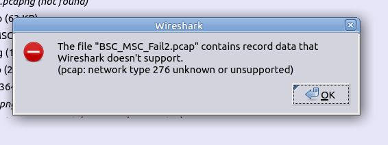
A lesson learned a long time ago in Net Eng, is that packet captures (seldom) lie, and the answers are almost always in the packets.
The issue is just getting those packets.
The Problem
But if you’re anything like me, you’re working on remote systems from your workstation, and trying to see what’s going on.
For me this goes like this:
SSH into machine in question
Start TCPdump
Hope that I have run it for long enough to capture the event of interest
Stop TCPdump
Change permissions on PCAP file created so I can copy it
SFTP into the machine in question
Transfer the PCAP to my local machine
View the PCAP in Wireshark
Discover I had not run the PCAP for long enough and repeat
Being a Mikrotik user I fell in love with the remote packet sniffer functionality built into them, where the switch/router will copy packets matching a filter and just stream them to the IP of my workstation.
If only there was something I could use to get this same functionality on remote machines – without named pipes, X11 forwarding or any of the other “hacky” solutions…
The Solution
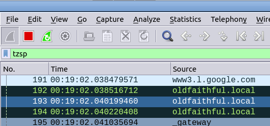
Introducing Scratch’n’Sniff, a simple tcpdump front end that encapsulates all the filtered traffic of interest in TZSP the same as Mikrotiks do, and stream it (in real time) to your local machine for real time viewing in Wireshark.
Using it is very simple:
Capture all traffic on port 5060 on interface enp0s25 and send it to 10.0.1.252 python3 scratchnsniff.py --dstip 10.0.1.252 --packetfilter 'port 5060' --interface enp0s25
Capture all sctp and icmp traffic on interface lo and send it to 10.98.1.2: python3 scratchnsniff.py --dstip 10.98.1.2 --packetfilter 'sctp or icmp' --interface lo
If you’re keen to try it out you can grab it from GitHub – Scratch’n’Sniff and start streaming packets remotely.
So you have a VoIP service and you want to rate the calls to charge your customers?
You’re running a mobile network and you need to meter data used by subscribers?
Need to do least-cost routing?
You want to offer prepaid mobile services?
Want to integrate with Asterisk, Kamailio, FreeSWITCH, Radius, Diameter, Packet Core, IMS, you name it!
Well friends, step right up, because today, we’re talking CGrates!
So before we get started, this isn’t going to be a 5 minute tutorial, I’ve a feeling this may end up a big multipart series like some of the others I’ve done. There is a learning curve here, and we’ll climb it together – but it is a climb.
Installation
Let’s start with a Debian based OS, installation is a doddle:
We’re going to use Redis for the DataDB and MariaDB as the StorDB (More on these concepts later), you should know that other backend options are available, but for keeping things simple we’ll just use these two.
Next we’ll get the database and config setup,
cd /usr/share/cgrates/storage/mysql/
./setup_cgr_db.sh root CGRateS.org localhost
cgr-migrator -exec=*set_versions -stordb_passwd=CGRateS.org
Lastly we’ll clone the config files from the GitHub repo:
In its simplest form, rating is taking a service being provided and calculating the cost for it.
The start of this series will focus on voice calls (With SMS, MMS, Data to come), where the callingparty (The person making the call) pays, so let’s imagine calling a Mobile number (Starting with 614) costs $0.22 per minute.
To perform rating we need to determine the Destination, the Rate to be applied, and the time to charge for.
For our example earlier, a call to a mobile (Any number starting with 614) should be charged at $0.22 per minute. So a 1 minute call will cost $0.22 and a 2 minute long call will cost $0.44, and so on.
We’ll also charge calls to fixed numbers (Prefix 612, 613, 617 and 617) at a flat $0.20 regardless of how long the call goes for.
So let’s start putting this whole thing together.
Introduction to RALs
RALs is the component in CGrates that takes care of Rating and Accounting Logic, and in this post, we’ll be looking at Rating.
The rates have hierarchical structure, which we’ll go into throughout this post. I took my notepad doodle of how everything fits together and digitized it below:
Destinations
Destinations are fairly simple, we’ll set them up in our Destinations.csv file, and it will look something like this:
Each entry has an ID (referred to higher up as the Destination ID), and a prefix.
Also notice that some Prefixes share an ID, for example 612, 613, 617 & 618 are under the Destination ID named “DST_AUS_Fixed”, so a call to any of those prefixes would match DST_AUS_Fixed.
Rates
Rates define the price we charge for a service and are defined by our Rates.csv file.
This is nice and clean, a 1 second call costs $0.25, a 60 second call costs $0.25, and a 61 second call costs $0.50, and so on.
This is the standard billing mechanism for residential services, but it does not pro-rata the call – For example a 1 second call is the same cost as a 59 second call ($0.25), and only if you tick over to 61 seconds does it get charged again (Total of $0.50).
Per Second Billing
If you’re doing a high volume of calls, paying for a 3 second long call where someone’s voicemail answers the call and was hung up, may seem a bit steep to pay the same for that as you would pay for 59 seconds of talk time.
Instead Per Second Billing is more common for high volume customers or carrier-interconnects.
This means the rate still be set at $0.25 per minute, but calculated per second.
So the cost of 60 seconds of call is $0.25, but the cost of 30 second call (half a minute) should cost half of that, so a 30 second call would cost $0.125.
How often we asses the charging is defined by the RateIncrement parameter in the Rate Table.
We could achieve the same outcome another way, by setting the RateIncriment to 1 second, and the dividing the rate per minute by 60, we would get the same outcome, but would be more messy and harder to maintain, but you could think of this as $0.25 per minute, or $0.004166667 per second ($0.25/60 seconds).
Flat Rate Billing
Another option that’s commonly used is to charge a flat rate for the call, so when the call is answered, you’re charged that rate, regardless of the length of the call.
Regardless if the call is for 1 second or 10 hours, the charge is the same.
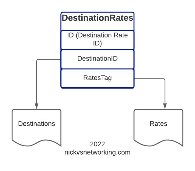
DestinationID – Refers to the DestinationID defined in the Destinations.csv file
RatesTag – Referes to the Rate ID we defined in Rates.csv
RoundingMethod – Defines if we round up or down
RoundingDecimals – Defines how many decimal places to consider before rounding
MaxCost – The maximum cost this can go up to
MaxCostStrategy – What to do if the Maximum Cost is reached – Either make the rest of the call Free or Disconnect the call
So for each entry we’ll define an ID, reference the Destination and the Rate to be applied, the other parts we’ll leave as boilerplate for now, and presto. We have linked our Destinations to Rates.
Rating Plans
We may want to offer different plans for different customers, with different rates.
DestinationRatesId (As defined in DestinationRates.csv)
TimingTag – References a time profile if used
Weight – Used to determine what precedence to use if multiple matches
So as you may imagine we need to link the DestinationRateIDs we just defined together into a Rating Plan, so that’s what I’ve done in the example above.
Rating Profiles
The last step in our chain is to link Customers / Subscribers to the profiles we’ve just defined.
How you allocate a customer to a particular Rating Plan is up to you, there’s numerous ways to approach it, but for this example we’re going to use one Rating Profile for all callers coming from the “cgrates.org” tenant:
Category is used to define the type of service we’re charging for, in this case it’s a call, but could also be an SMS, Data usage, or a custom definition.
Subject is typically the calling party, we could set this to be the Caller ID, but in this case I’ve used a wildcard “*any”
ActivationTime allows us to define a start time for the Rating Profile, for example if all our rates go up on the 1st of each month, we can update the Plans and add a new entry in the Rating Profile with the new Plans with the start time set
RatingPlanID sets the Rating Plan that is used as we defined in RatingPlans.csv
Loading the Rates into CGrates
At the start we’ll be dealing with CGrates through CSV files we import, this is just one way to interface with CGrates, there’s others we’ll cover in due time.
CGRates has a clever realtime architecture that we won’t go into in any great depth, but in order to load data in from a CSV file there’s a simple handy tool to run the process,
Obviously you’ll need to replace with the folder you cloned from GitHub.
Trying it Out
In order for CGrates to work with Kamailio, FreeSWITCH, Asterisk, Diameter, Radius, and a stack of custom options, for rating calls, it has to have common mechanisms for retrieving this data.
CGrates provides an API for rating calls, that’s used by these platforms, and there’s a tool we can use to emulate the signaling for call being charged, without needing to pickup the phone or integrate a platform into it.
The tenant will need to match those defined in the RatingProfiles.csv, the Subject is the Calling Party identity, in our case we’re using a wildcard match so it doesn’t matter really what it’s set to, the Destination is the destination of the call, AnswerTime is time of the call being answered (pretty self explanatory) and the usage defines how many seconds the call has progressed for.
The output is a JSON string, containing a stack of useful information for us, including the Cost of the call, but also the rates that go into the decision making process so we can see the logic that went into the price.
So have a play with setting up more Destinations, Rates, DestinationRates and RatingPlans, in these CSV files, and in our next post we’ll dig a little deeper… And throw away the CSVs all together!
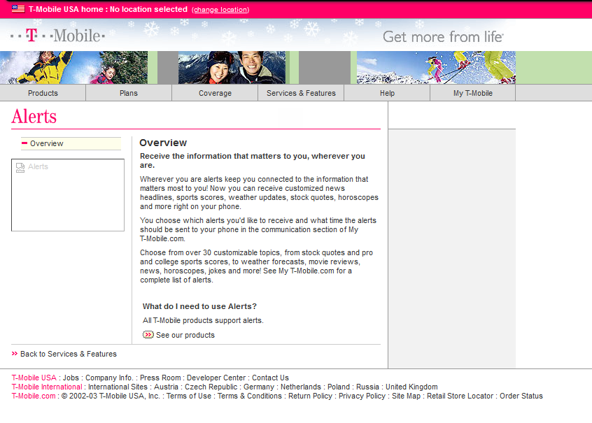
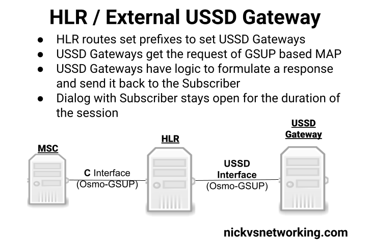
Unstructured Supplementary Service Data or “USSD” is the stack used in Cellular Networks to offer interactive text based menus and systems to Subscribers.
If you remember topping up your mobile phone credit via a text menu on your flip phone, there’s a good chance that was USSD*.
For a period, USSD Services provided Sporting Scores, Stock Prices and horoscopes on phones and networks that were not enabled for packet data.
Unlike plain SMS-PP, USSD services are transaction stateful, which means that there is a session / dialog between the subscriber and the USSD gateway that keeps track of the session and what has happened in the session thus far.
T-Mobile website from 2003 covering the features of their USSD based product at the time
Today USSD is primarily used in the network at times when a subscriber may not have balance to access packet data (Internet) services, so primarily is used for recharging with vouchers.
Osmocom’s HLR (osmo-hlr) has an External USSD interface to allow you to define the USSD logic in another entity, for example you could interface the USSD service with a chat bot, or interface with a billing system to manage credit.
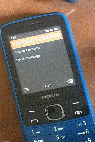
Using the example code provided I made a little demo of how the service could be used:
Communication between the USSD Gateway and the HLR is MAP but carried GSUP (Rather than the full MTP3/SCCP/TCAP layers that traditionally MAP stits on top of), and inside the HLR you define the prefixes and which USSD Gateway to route them to (This would allow you to have multiple USSD gateways and route the requests to them based on the code the subscriber sends).
(I had hoped to make a Python example and actually interface it with some external systems, but another day!)
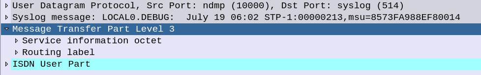
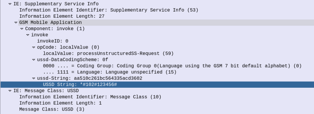
The signaling is fairly straight forward, when the subscriber kicks off the USSD request, the HLR calls a MAP Invoke operation for “processUnstructuredSS-Request”
Unfortunately is seems the stock Android does not support interactive USSD. This is exposed in the Android SDK so applications can access USSD interfaces (including interactive USSD) but the stock dialer on the few phones I played with did not, which threw a bit of a spanner in the works. There are a few apps that can help with this however I didn’t go into any of them.
(or maybe they used SIM Toolkit which had a similar interface)
So I run a lot of VMs. It’s not unusual when I’m automating something with Ansible or setting up a complex lab to be running 20+ VMs at a time, and often I’ll create a base VM and clone it a dozen times.
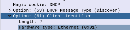
Alas, Ubuntu 20.04 has some very irritating default behaviour, where even if the MAC addresses of these cloned VMs differ they get the same IP Address from DHCP.
That’s because by default Netplan doesn’t use the MAC address as the identifier when requesting a DHCP lease. And if you’ve cloned a VM the identifier it does use doesn’t change even if you do change the MAC address…
Irritating, but easily fixed!
Editing the netplan config:
network:
  ethernets:
    eth0:
      dhcp4: true
      dhcp-identifier: mac
  version: 2
Run a netplan-apply and you’re done.
Now you can clone that VM as many times as you like and each will get it’s own unique IP address.
This is part of a series of posts looking into SS7 and Sigtran networks. We cover some basic theory and then get into the weeds with GNS3 based labs where we will build real SS7/Sigtran based networks and use them to carry traffic.
Having a direct Linkset from every Point Code to every other Point Code in an SS7 network isn’t practical, we need to rely on routing, so in this post we’ll cover routing between Point Codes on our STPs.
Let’s start in the IP world, imagine a router with a routing table that looks something like this:
Simple IP Routing Table
192.168.0.0/24 out 192.168.0.1 (Directly Attached)
172.16.8.0/22 via 192.168.0.3 - Static Route - (Priority 100)
172.16.0.0/16 via 192.168.0.2 - Static Route - (Priority 50)
10.98.22.1/32 via 192.168.0.3 - Static Route - (Priority 50)
We have an implicit route for the network we’re directly attached to (192.168.0.0/24), and then a series of static routes we configure. We’ve also got two routes to the 172.16.8.0/22 subnet, one is more specific with a higher priority (172.16.8.0/22 – Priority 100), while the other is less specific with a lower priority (172.16.0.0/16 – Priority 50). The higher priority route will take precedence.
This should look pretty familiar to you, but now we’re going to take a look at routing in SS7, and for that we’re going to be talking Variable Length Subnet Masking in detail you haven’t needed to think about since doing your CCNA years ago…
Why Masking is Important
A route to a single Point Code is called a “/14”, this is akin to a single IPv4 address being called a “/32”.
We could setup all our routing tables with static routes to each point code (/14), but with about 4,000 international point codes, this might be a challenge.
Instead, by using Masks, we can group together ranges of Point Codes and route those ranges through a particular STP.
This opens up the ability to achieve things like “Route all traffic to Point Codes to this Default Gateway STP”, or to say “Route all traffic to this region through this STP”.
Individually routing to a point code works well for small scale networking, but there’s power, flexibility and simplification that comes from grouping together ranges of point codes.
Information Overload about Point Codes
So far we’ve talked about point codes in the X.YYY.Z format, in our lab we setup point codes like 1.2.3.
This is not the only option however…
Variants of SS7 Point Codes
IPv4 addresses look the same regardless of where you are. From Algeria to Zimbabwe, IPv4 addresses look the same and route the same.
In SS7 networks that’s not the case – There are a lot of variants that define how a point code is structured, how long it is, etc. Common variants are ANSI, ITU-T (International & National variants), ETSI, Japan NTT, TTC & China.
The SS7 variant used must match on both ends of a link; this means an SS7 node speaking ETSI flavoured Point Codes can’t exchange messages with an ANSI flavoured Point Code.
Well, you can kinda translate from one variant to another, but requires some rewriting not unlike how NAT does it.
ITU International Variant
For the start of this series, we’ll be working with the ITU International variant / flavour of Point Code.
ITU International point codes are 14 bits long, and format is described as 3-8-3. The 3-8-3 form of Point code just means the 14 bit long point code is broken up into three sections, the first section is made up of the first 3 bits, the second section is made up of the next 8 bits then the remaining 3 bits in the last section, for a total of 14 bits.
So our 14 bit 3-8-3 Point Code looks like this in binary form:
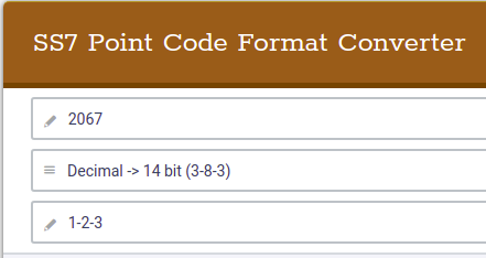
If you’re dealing with multiple vendors or products,you’ll see some SS7 Point Codes represented as decimal (2067), some showing as 1-2-3 codes and sometimes just raw binary. Fun hey?
So why does the binary part matter? Well the answer is for masks.
To loop back to the start of this post, we talked about IP routing using a network address and netmask, to represent a range of IP addresses. We can do the same for SS7 Point Codes, but that requires a teeny bit of working out.
As an example let’s imagine we need to setup a route to all point codes from 3-4-0 through to 3-6-7, without specifying all the individual point codes between them.
Firstly let’s look at our start and end point codes in binary:
100-00000100-000 = 3-004-0 (Start Point Code)
100-00000110-111 = 3-006-7 (End Point Code)
Looking at the above example let’s look at how many bits are common between the two,
100-00000100-000 = 3-004-0 (Start Point Code)
100-00000110-111 = 3-006-7 (End Point Code)
The first 9 bits are common, it’s only the last 5 bits that change, so we can group all these together by saying we have a /9 mask.
When it comes time to add a route, we can add a route to 3-4-0/9 and that tells our STP to match everything from point code 3-4-0 through to point code 3-6-7.
The STP doing the routing it only needs to match on the first 9 bits in the point code, to match this route.
SS7 Routing Tables
Now we have covered Masking for roues, we can start putting some routes into our network.
In order to get a message from one point code to another point code, where there isn’t a direct linkset between the two, we need to rely on routing, which is performed by our STPs.
This is where all that point code mask stuff we just covered comes in.
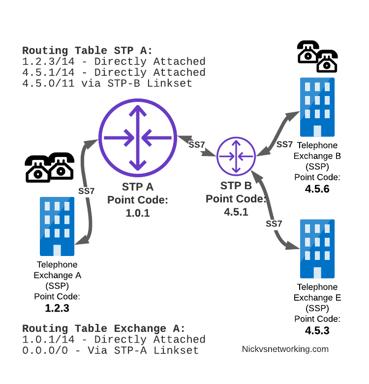
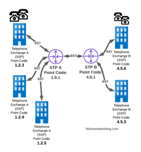
Let’s look at a diagram below,
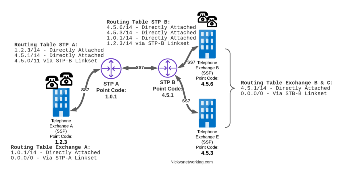
Let’s look at the routing to get a message from Exchange A (SSP) on the bottom left of the picture to Exchange E (SSP) with Point Code 4.5.3 in the bottom right of the picture.
Exchange A (SSP) on the bottom left of the picture has point code 1.2.3 assigned to it and a Linkset to STP-A. It has the implicit route to STP-A as it’s got that linkset, but it’s also got a route configured on it to reach any other point code via the Linkset to STP-A via the 0.0.0/0 route which is the SS7 equivalent of a default route. This means any traffic to any point code will go to STP-A.
From STP-A we have a linkset to STP-B. In order to route to the point codes behind STP-B, STP-A has a route to match any Point Code starting with 4.5.X, which is 4.5.0/11. This means that STP-A will route any Point Code between 4.5.1 and 4.5.7 down the Linkset to STP-B.
STP-B has got a direct connection to Exchange B and Exchange E, so has implicit routes to reach each of them.
So with that routing table, Exchange A should be able to route a message to Exchange E.
But…
Return Routing
Just like in IP routing, we need return routing. while Exchange A (SSP) at 1.2.3 has a route to everywhere in the network, the other parts of the network don’t have a route to get to it. This means a request from 1.2.3 can get anywhere in the network, but it can’t get a response back to 1.2.3.
So to get traffic back to Exchange A (SSP) at 1.2.3, our two Exchanges on the right (Exchange B & C with point codes 4.5.6 and 4.5.3) will need routes added to them. We’ll also need to add routes to STP-B, and once we’ve done that, we should be able to get from Exchange A to any point code in this network.
There is a route missing here, see if you can pick up what it is!
So we’ve added a default route via STP-B on Exchange B & Exchange E, and added a route on STP-B to send anything to 1.2.3/14 via STP-A, and with that we should be able to route from any exchange to any other exchange.
One last point on terminology – when we specify a route we don’t talk in terms of the next hop Point Code, but the Linkset to route it down. For example the default route on Exchange A is 0.0.0/0 via STP-A linkset (The linkset from Exchange A to STP-A), we don’t specify the point code of STP-A, but just the name of the Linkset between them.
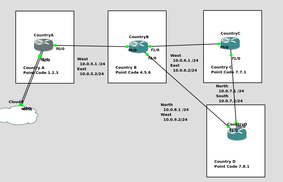
Back into the Lab
So back to the lab, where we left it was with linksets between each point code, so each Country could talk to it’s neighbor.
Let’s confirm this is the case before we go setting up routes, then together, we’ll get a route from Country A to Country C (and back).
So let’s check the status of the link from Country B to its two neighbors – Country A and Country C. All going well it should look like this, and if it doesn’t, then stop by my last post and check you’ve got everything setup.
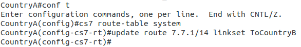
So let’s add some routing so Country A can reach Country C via Country B. On Country A STP we’ll need to add a static route. For this example we’ll add a route to 7.7.1/14 (Just Country C).
That means Country A knows how to get to Country C. But with no return routing, Country C doesn’t know how to get to Country A. So let’s fix that.
We’ll add a static route to Country C to send everything via Country B.
CountryC#conf t
Enter configuration commands, one per line.  End with CNTL/Z.
CountryC(config)#cs7 route-table system
CountryC(config)#update route 0.0.0/0 linkset ToCountryB
*Jan 01 05:37:28.879: %CS7MTP3-5-DESTSTATUS: Destination 0.0.0 is accessible
So now from Country C, let’s see if we can ping Country A (Ok, it’s not a “real” ICMP ping, it’s a link state check message, but the result is essentially the same).
By running:
CountryC# ping cs7 1.2.3
*Jan 01 06:28:53.699: %CS7PING-6-RTT: Test Q.755 1.2.3: MTP Traffic test rtt 48/48/48
*Jan 01 06:28:53.699: %CS7PING-6-STAT: Test Q.755 1.2.3: MTP Traffic test 100% successful packets(1/1)
*Jan 01 06:28:53.699: %CS7PING-6-RATES: Test Q.755 1.2.3: Receive rate(pps:kbps) 1:0 Sent rate(pps:kbps) 1:0
*Jan 01 06:28:53.699: %CS7PING-6-TERM: Test Q.755 1.2.3: MTP Traffic test terminated.
We can confirm now that Country C can reach Country A, we can do the same from Country A to confirm we can reach Country B.
But what about Country D? The route we added on Country A won’t cover Country D, and to get to Country D, again we go through Country B.
This means we could group Country C and Country D into one route entry on Country A that matches anything starting with 7-X-X,
For this we’d add a route on Country A, and then remove the original route;
Of course, you may have already picked up, we’ll need to add a return route to Country D, so that it has a default route pointing all traffic to STP-B. Once we’ve done that from Country A we should be able to reach all the other countries:
CountryA#show cs7 route
Dynamic Routes 0 of 1000

Routing table = system Destinations = 3 Routes = 3

Destination            Prio Linkset Name        Route
---------------------- ---- ------------------- -------
4.5.6/14         acces   1  ToCountryB          avail
7.0.0/3          acces   5  ToCountryB          avail


CountryA#ping cs7 7.8.1
*Jan 01 07:28:19.503: %CS7PING-6-RTT: Test Q.755 7.8.1: MTP Traffic test rtt 84/84/84
*Jan 01 07:28:19.503: %CS7PING-6-STAT: Test Q.755 7.8.1: MTP Traffic test 100% successful packets(1/1)
*Jan 01 07:28:19.503: %CS7PING-6-RATES: Test Q.755 7.8.1: Receive rate(pps:kbps) 1:0  Sent rate(pps:kbps) 1:0
*Jan 01 07:28:19.507: %CS7PING-6-TERM: Test Q.755 7.8.1: MTP Traffic test terminated.
CountryA#ping cs7 7.7.1
*Jan 01 07:28:26.839: %CS7PING-6-RTT: Test Q.755 7.7.1: MTP Traffic test rtt 60/60/60
*Jan 01 07:28:26.839: %CS7PING-6-STAT: Test Q.755 7.7.1: MTP Traffic test 100% successful packets(1/1)
*Jan 01 07:28:26.839: %CS7PING-6-RATES: Test Q.755 7.7.1: Receive rate(pps:kbps) 1:0  Sent rate(pps:kbps) 1:0
*Jan 01 07:28:26.843: %CS7PING-6-TERM: Test Q.755 7.7.1: MTP Traffic test terminated.
So where to from here?
Well, we now have a a functional SS7 network made up of STPs, with routing between them, but if we go back to our SS7 network overview diagram from before, you’ll notice there’s something missing from our lab network…
So far our network is made up only of STPs, that’s like building a network only out of routers!
In our next lab, we’ll start adding some SSPs to actually generate some SS7 traffic on the network, rather than just OAM traffic.
Chances are if you’re reading this, you’re trying to work out what Telephony Binary-Coded Decimal encoding is. I got you.
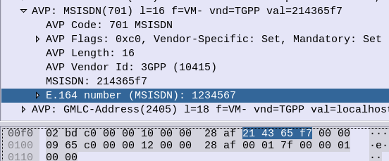
Again I found myself staring at encoding trying to guess how it worked, reading references that looped into other references, in this case I was encoding MSISDN AVPs in Diameter.
How to Encode a number using Telephony Binary-Coded Decimal encoding?
First, Group all the numbers into pairs, and reverse each pair.
So a phone number of 123456, becomes:
214365
Because 1 & 2 are swapped to become 21, 3 & 4 are swapped to become 34, 5 & 6 become 65, that’s how we get that result.
TBCD Encoding of numbers with an Odd Length?
If we’ve got an odd-number of digits, we add an F on the end and still flip the digits,
For example 789, we add the F to the end to pad it to an even length, and then flip each pair of digits, so it becomes:
87F9
That’s the abbreviated version of it. If you’re only encoding numbers that’s all you’ll need to know.
Detail Overload
Because the numbers 0-9 can be encoded using only 4 bits, the need for a whole 8 bit byte to store this information is considered excessive.
For example 1 represented as a binary 8-bit byte would be 00000001, while 9 would be 00001001, so even with our largest number, the first 4 bits would always going to be 0000 – we’d only use half the available space.
So TBCD encoding stores two numbers in each Byte (1 number in the first 4 bits, one number in the second 4 bits).
To go back to our previous example, 1 represented as a binary 4-bit word would be 0001, while 9 would be 1001. These are then swapped and concatenated, so the number 19 becomes 1001 0001 which is hex 0x91.
Let’s do another example, 82, so 8 represented as a 4-bit word is 1000 and 2 as a 4-bit word is 0010. We then swap the order and concatenate to get 00101000 which is hex 0x28 from our inputted 82.
Final example will be a 3 digit number, 123. As we saw earlier we’ll add an F to the end for padding, and then encode as we would any other number,
F is encoded as 1111.
1 becomes 0001, 2 becomes 0010, 3 becomes 0011 and F becomes 1111. Reverse each pair and concatenate 00100001 11110011 or hex 0x21 0xF3.
Special Symbols (#, * and friends)
Because TBCD Encoding was designed for use in Telephony networks, the # and * symbols are also present, as they are on a telephone keypad.
Astute readers may have noticed that so far we’ve covered 0-9 and F, which still doesn’t use all the available space in the 4 bit area.
The extended DTMF keys of A, B & C are also valid in TBCD (The D key was sacrificed to get the F in).
Symbol
4 Bit Word
*
1 0 1 0
#
1 0 1 1
a
1 1 0 0
b
1 1 0 1
c
1 1 1 0
So let’s run through some more examples,
*21 is an odd length, so we’ll slap an F on the end (*21F), and then encoded each pair of values into bytes, so * becomes 1010, 2 becomes 0010. Swap them and concatenate for our first byte of 00101010 (Hex 0x2A). F our second byte 1F, 1 becomes 0001 and F becomes 1111. Swap and concatenate to get 11110001 (Hex 0xF1). So *21 becomes 0x2A 0xF1.
And as promised, some Python code from PyHSS that does it for you:
    def TBCD_special_chars(self, input):
        if input == "*":
            return "1010"
        elif input == "#":
            return "1011"
        elif input == "a":
            return "1100"
        elif input == "b":
            return "1101"
        elif input == "c":
            return "1100"
        else:
            print("input " + str(input) + " is not a special char, converting to bin ")
            return ("{:04b}".format(int(input)))


    def TBCD_encode(self, input):
        print("TBCD_encode input value is " + str(input))
        offset = 0
        output = ''
        matches = ['*', '#', 'a', 'b', 'c']
        while offset < len(input):
            if len(input[offset:offset+2]) == 2:
                bit = input[offset:offset+2]    #Get two digits at a time
                bit = bit[::-1]                 #Reverse them
                #Check if *, #, a, b or c
                if any(x in bit for x in matches):
                    new_bit = ''
                    new_bit = new_bit + str(TBCD_special_chars(bit[0]))
                    new_bit = new_bit + str(TBCD_special_chars(bit[1]))
                    bit = str(int(new_bit, 2))
                output = output + bit
                offset = offset + 2
            else:
                bit = "f" + str(input[offset:offset+2])
                output = output + bit
                print("TBCD_encode output value is " + str(output))
                return output


    def TBCD_decode(self, input):
        print("TBCD_decode Input value is " + str(input))
        offset = 0
        output = ''
        while offset < len(input):
            if "f" not in input[offset:offset+2]:
                bit = input[offset:offset+2]    #Get two digits at a time
                bit = bit[::-1]                 #Reverse them
                output = output + bit
                offset = offset + 2
            else:   #If f in bit strip it
                bit = input[offset:offset+2]
                output = output + bit[1]
                print("TBCD_decode output value is " + str(output))
                return output
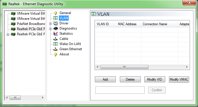
Just discovered you can add VLANs to Realtek NICs on Windows PCs,
I have a fairly grunty desktop I use for running anything that needs Windows, running VMware Workstation and occasional gaming,
I do have a big Dell machine running ESXi which supports VLAN tagging and trunking, but I try and avoid using it as it’s deafeningly loud and very power hungry.
Recently as the lab network I use grows and grows I’ve been struggling to run all the VMs running in Workstation as I’ve been running out of IP space and wanting some more separation between networks.
Now I can add VLANs onto the existing NIC using the Realtek Ethernet Diagnostic Utility, and then bridge each of these NICs to the respective VM in Workstation, and the port to the Mikrotik CRS is now a trunk with all the VLANs on it.
As Open5Gs has introduced network slicing, which led to a change in the database used,
Alas many users had subscribers provisioned in the old DB schema and no way to migrate the SDM data between the old and new schema,
If you’ve created subscribers on the old schema, and now after the updates your Subscriber Authentication is failing, check out this tool I put together, to migrate your data over.
I’d been trying for some time to get Kamailio acting as a Diameter Routing Agent with mixed success, and eventually got it working, after a few changes to the codebase of the ims_diameter_server module.
It is rather unstable, in that if it fails to dispatch to a Diameter peer, the whole thing comes crumbling down, but incoming Diameter traffic is proxied off to another Diameter peer, and Kamailio even adds an extra AVP.
Having used Kamailio for so long I was really hoping I could work with Kamailio as a DRA as easily as I do for SIP traffic, but it seems the Diameter module still needs a lot more love before it’ll be stable enough and simple enough for everyone to use.
I created a branch containing the fixes I made to make it work, and with an example config for use, but use with caution. It’s a long way from being production-ready, but hopefully in time will evolve.