Sometimes I wonder how much crack kit vendors and operator’s marketing teams smoke, and if they ever talk to end users.
I was reading about 5G eRedcap the other day – how it is the next generation of 5G Redcap (reduced capacity – a subset of the UE standard with a cut down feature set to make them cheaper to produce / more power efficient), which is in itself a subset of 5G SA for IoT devices.
One of the key pillars 5G SA promised is MmTC (Massive Machine Type Communication) which just means IoT but that’s separate to Redcap and eRedcap.
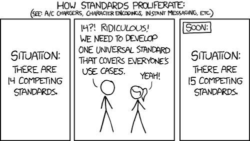
Did I mention none are compatible with each other and some are mutually exclusive.
All this is is great because in 4G we had wideband LTE (standard LTE) but also NB-IoT (Aka Narrowband) and also Cat-M1.
So clear and easy to understand.
If you’re designing an IoT enabled rat trap, water meter or widget production line, before you pick the modem to go in your device, you need to know about what IoT technologies are available on what bands from what operators in countries you haven’t even considered selling into yet.
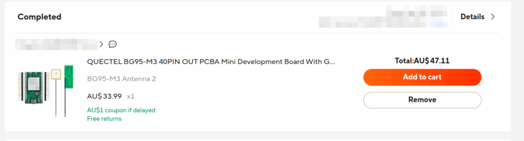
This has been in the front of my mind of late; I’ve been messing around with LTE NB-IoT, so I thought I’d find a dev board that supports NB-IoT (a standard that’s now almost 10 years old) so I can validate it all works.
The cheapest NB-IoT capable dev board I could find used a Quectel chipset, BG95-M3, and it cost me $47 AUD (~$30 USD).
By contrast, I can buy a GSM modem on a breakout board in single quantities for $3.50 USD.
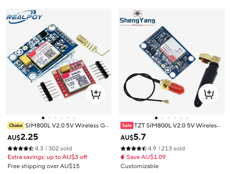
There’s a tension here – the cellular industry desperately tries to sunset old tech (because it’s expensive for them to operate), and those building IoT devices are incentiviced to use the cheapest modems for their application – so use the 2G modems because they’re 1/6th the price because it’s cheaper for them to build.
Years ago a family member had purchased a bunch of 2G trailcams, which stopped working when Australia shut off the 2G network. The result is the consumer’s previously working hardware has now stopped working. The vendor washes their hands of it – they can’t control what the operators do, and the operators say they can’t stand in the way of progress, and the consumer just ends up with eWaste and a bad taste in their mouth.
So why is a 2G modem so dammed cheap? Mostly it’s just economies of scale. There’s a handful of GSM bands, and one technology – GSM.
If you’re Qualcomm, SIMcomm, Quectel or any of the other chip vendors, you want to build one chip and sell it to the largest possible market, a good example was the $10 USD USB modems that run Android I wrote about last year.
But for IoT, these more obscure cellular standards are fragmented, with different bands and technologies across multiple operators even in the same country, and that doesn’t scale well to have multiple different SKUs for slight variations in the same product.
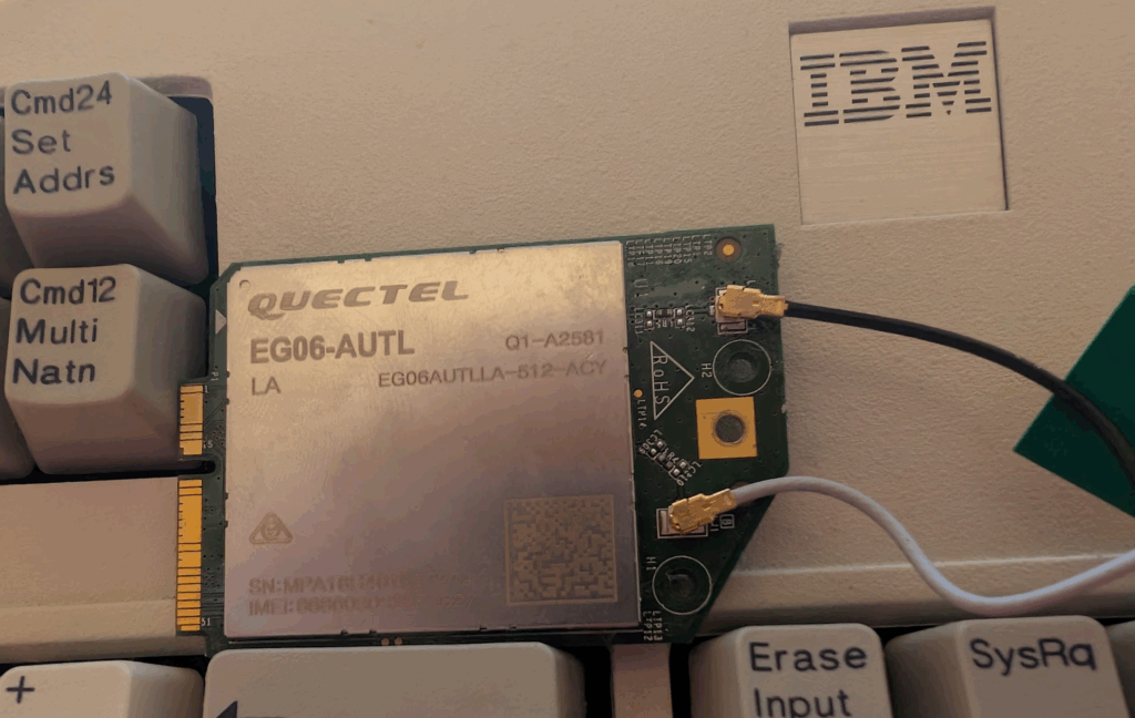
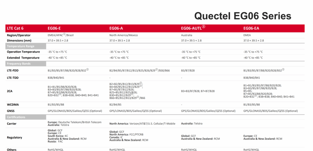
Here’s a random Quectel chip on my desk I pulled out of a modem, it’s the EG06-AUTL, which if we look at the datasheet is the Australian variant, only for Telstra, but the EG06-E would work for Australia too, but not the EG06-EA or EG06-A (Yes, this isn’t strictly an IoT chip but you get the point).
WiFi chips like the ubiquitous ESP8266 are under $2 USD, have no ongoing monthly and work anywhere in the world. If I need more range a LoRa module costs ~$5 USD and has no reliance on local cellular networks, and again, no ongoing subscription. And with WiFi and LoRa, no one can unilaterally say “We’re turning off this network”.
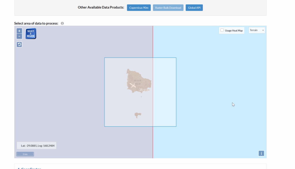
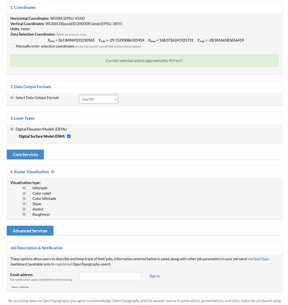
A few years ago I did some work on an island where we replaced dial up modem banks belonging to the local water corporation with LTE Routers connected to an LTE network we’d helped build.
The water monitoring kit talked Modbus from the 1970s and didn’t give a stuff about if it was going on LTE or point to point dial up links – it was like the wise old turtle who’d seen standards come and go.
If you’ve read this far maybe you’re expecting some call to action or deep insight, maybe you’ve been reading this blog long enough to know not to expect such things from me. The more I think about it the more I wonder if the cellular industry should just give up on IoT.
The ARPUs for IoT are minuscule, the cost to deliver is high and there are a multitude of competing technologies out there.
I’m not suggesting exiting the space entirely, but when it’s cheaper to buy a full fat LTE modem then an LTE NB-IoT modem, the use case for having a dedicated subset of a standard like NB-IoT or Redcap could be scrapped – If device manufacturers want cellular, they include full cellular, and if they want low power, long battery life, etc, they go Lora or WiFi or any of the other competing standards they were going to pick anyway.