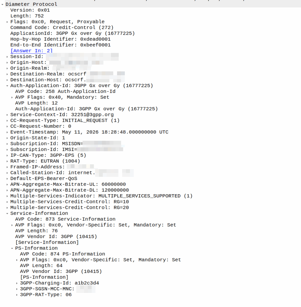
I was recently asked by a potential customer if we supported Gx over Gy.
I’d never heard of this before, so I gave my standard “If it’s in the spec we should support it, but I’ll check” answer, and got them to send me a PCAP, which I’ve got.
This is weird.
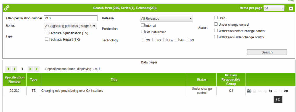
So for starers, Protocoldex has nothing for this application ID (16777225), even though it has all the LTE diameter specs.
The last version was from 2006, in 3GPP release 6, which is two years before LTE was standardized in Release 8. The word LTE does not appear in the doc or in the metadata tags.
It speaks of TPF (Traffic Plane Function) and TPF (Charging Rules Function).
LTE is “Long Term Evolution” – In later releases this draft TPF would evolve into the PGW (before the PGW-C / PGW-U divorce) and the TPF would go on to become the PCRF (and save spring break).
Reading through these early specs is like looking at Homo Eructs (get your mind out of the gutter) and knowing it evolves into Homo Sapiens.
So what does Gx over Gy do? Well, the concept is pretty straightforward, rather than needing a Sy interface between the PCRF and OCS, you can provision policy rules from the OCS, rather than on the PCRF.
So what network functions should implement this standard? Well, the P-GW specs do not reference this as something that’s included in the P-GW, nor is it in the GGSN – This was a “gooch” spec between the hypothetical standards land and real world implementations.
So will we be implementing it? Probably not. But an interesting bit of archaeology and a look through the genealogy of 3GPP.
This is an idea I’ve been kicking around for a little while – A single GSM TRX being broadcast across multiple cell sites.
Generally in GSM land, a “TRX” is a cell or a sector – but it doesn’t need to be. Later in GSM features like antenna diversity allow the same signal to be broadcast out multiple ports and received on multiple ports, and these to even work together.
Knowing this is possible, what if you run a single TRX across multiple cells / sectors / sites?
This means rather than cell site A & cell site B being “neighbors” they’re a single TRX. A subscriber moving between the two sees the same LAC and Cell ID, but they see the signal strength drop and then rise as they move between the cells, but there’s no “handover” – it’d look to the phone the same as going away from a cell then coming closer, which is what they’ve done, but the cell is being broadcast from two locations.
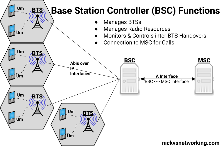
So why do this? Well, while VoLTE is nice, handset support on low end feature phones is still shite, and it means in some of the places we operate we couldn’t capture the low end of the market – those who just needed a basic voice service. As such we’ve finallyadded an MSC to our product offering (after almost 10 years of me swearing there’s no way we’d build legacy crap) and a BSC that’s compatible with our existing RAN portfolio (Nokia Airscale), all to be able to address that gap, by running a small GSM layer off our existing radios.
The capacity would be shared of course – this is just one TRX, so 8 full rate channels, but for our use of CSFB for feature phones, garbage IoT devices, it doesn’t matter. On spectral efficiency this is way better than a 5Mhz UMTS carrier (smallest you can do) and co-exists nicely with LTE.
Running a large number of sectors / cells on a common single TRX means when you’ve got a boundary where you need to hand to another TRX, you need fewer channels your reuse pattern. Even running 3 TRXes in our “Super cell” area, is only 600Khz of bandwidth consumed, and if the area is large enough we can do a ~3:1 reuse pattern.
For this to work we’ve got to serve all the cells of a single baseband, but baseband hotels are becoming the norm, and fiber is everywhere. I did start exploring if we could do one TRX on multiple BTSes on our BSC, from an Abis perspective it’d work, but we’d need to ensure timing and I don’t know enough about how the clocking works on our BTSes to say for sure that they’d be in sync even with GLONASS/GPS.
Would this work at scale? I’ve no idea, but I’m hoping to find out!
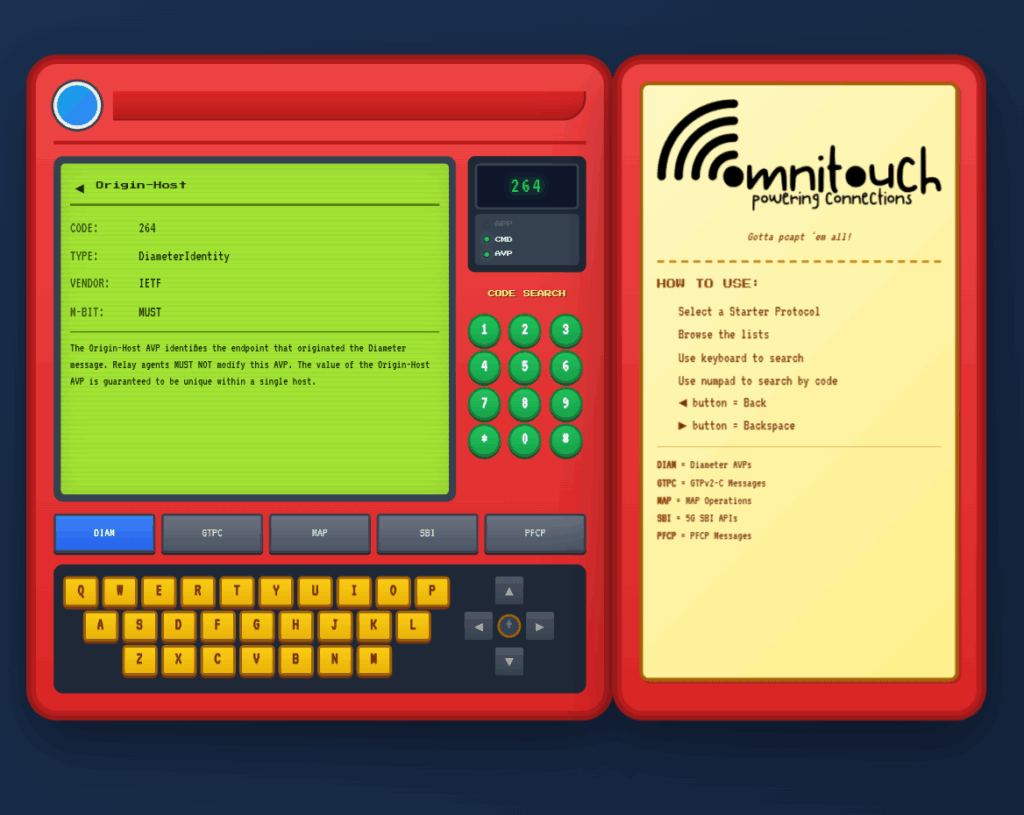
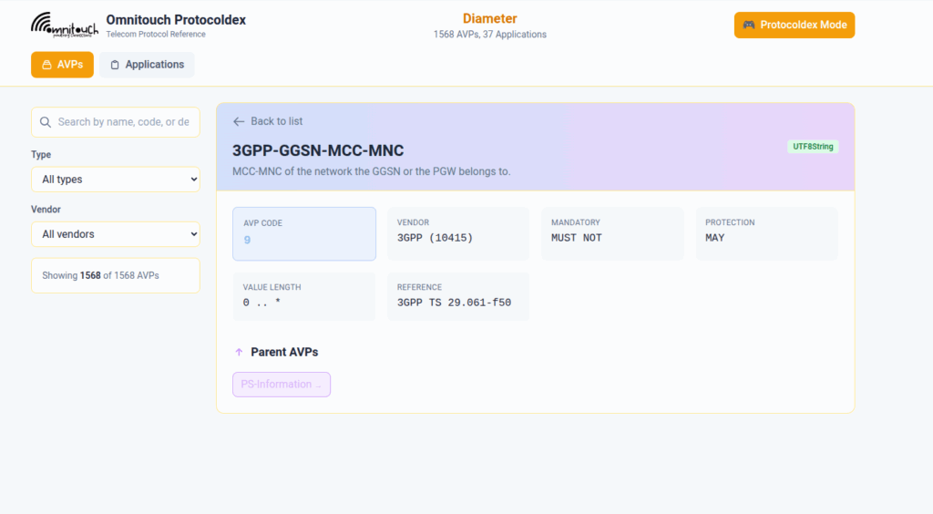
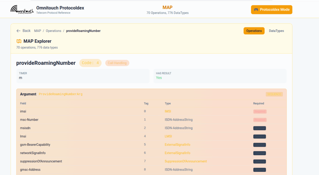
I do a lot of protocol testing, writing Diameter/PFCP/GTP-C etc, and spend a lot of time referencing the standards.
So I built this – Inspired by a 1990s video game / TV / Playing card franchise online reference tool, but rather than identifying pocket monsters, it’s identifying AVPs and stuff
You can punch in the AVP code, AVP name, description, etc, for Diameter, PFCP, GTP-C, MAP or SBI and see all the details to go with it.
I’ve been using it a heap, hopefully some of you might find it useful:
One of our customers is an MVNE and they reached out the other day with an issue.
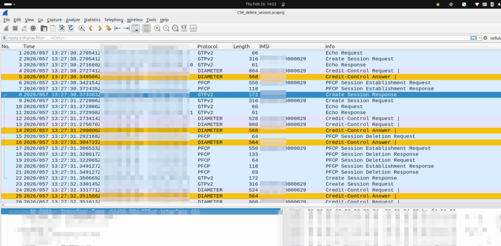
They were turning up a new PGW and they’d see Create Session Request, everything looked OK, it’d get a response, but then in the GUI of the PGW-C they’d see the session drop.
The logs showed the newly setup session dropping shortly after being setup.
Have a look at the screenshot and see if you can work out why:
So what’s going on, and why is the PGW-C deleting sessions?
The initial reaction from the customer was there’s something up with the PGW, but the answer is bit more nuanced.
Per the specs, you can’t have two PDN sessions for the same subscriber (IMSI) on the same APN (DNN).
So if 50557000000001 is connected to the PGW-C on the internet APN, if I send another Create Session Request to the same PGW-C, it deletes the old session, before starting the new one.
In this case, the MVNE it was going through was dropping the Create Session Response, so it never made it back to the MNO, and then the MME in the MNO sent it again.
Joys of GTPv2-C being UDP based and connectionless!
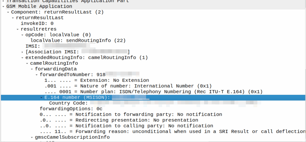
I’ve covered how SS7/ISUP handles call forward before, but the HLR can also store call forwarding information.
This is returned to the MSC when the SendRoutingInfo dialog is performed against the HLR.
If it’s present the MSC will redirect the call to that destination, after bouncing it through CAMEL (if enabled).
A lot simpler than Call Forward in IMS, but same outcome.
A lot of HSSes we see are just HLRs under the hood and only implement a minimalist MMTel feature set for call forwarding for this reason to have it track across both.
SMSc can send an SRI-for-SM, and if the subscriber is absent, the response can include the informServiceCenter message, which lets the SMSc know if it will get sent an alertServiceCentre message when the subscriber comes back online (sends an UpdateLocation).
This means that the SMSc can be notified when it can deliver the message to the subscriber.
It’s got a bunch of flags, which equate to:
sc-AddressNotIncluded means the service center address from the SRI-for-SM was not included in the Message Waiting Data file (and therefore will not get notified via AlertSC when the subscriber comes back online).
If it’s sc-AddressNotIncluded is set to False it means that the service center address has been added to the Message Waiting Data file, so will get an alertServiceCenter message when the sub comes back online (Double negative).
mnrf-Set means Mobile subscriber Not Reachable (Not registered on any MSC)
mcef-Set means Memory Capacity Exceeded Flag is set as the HLR has run out of memory in the Message Waiting Data file and cannot store any more data (So you won’t get notified via AlertSC when the subscriber comes back online)
mnrg-Set is for Mobile subscriber Not Reachable for GPRS (When using SGSN delivery is not registered for packet service).
mnr5g-Set means the SC will get notified when the subscriber becomes reachable from 5G serving nodes.
mnr5gn3g is a mystery – The only references to it I can find are in the ASN1 spec (hence why Wireshark decodes it) but as to its purpose, I can only guess.
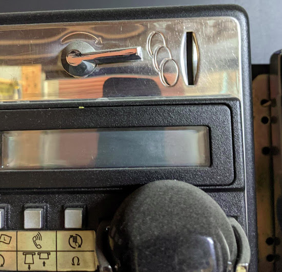
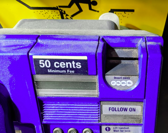
Let’s imagine the coin slot on a payphone – Coins can only enter the slot if they’re aligned with the slot.
If you tried to rotate the coin by 90 degrees, it wouldn’t fit it in the slot.
If the slot on the payphone went from up-to-down, our coin slot could be described as “vertically polarized”. Only coins in the vertically polarized orientation would fit.
Likewise, a payphone with the coin slot going side-to-side we could describe the coin slot as being “horizontally polarized”, meaning only coins that are horizontally polarized (on their side) would fit into the coin slot.
RF waves also have a polarization, like our coin slot.
A receiver wishing to receive into signals transmitted from a vertically-polarized antenna, will need to use a vertically-polarised antenna to pick up the signal.
Likewise a signal transmitted from a horizontally polarized antenna, would require a horizontally polarised antenna on the receiving side.
If there is a mismatch in polarization (for example RF waves transmitted from a horizontal polarized antenna but the receiver is using a vertically polarized antenna) the signal may still get through, but received signal strength would be severely degraded – in the order of 20dB, which is 1/100th of the power you’d get with the correct polarization.
You can think of polarization mismatches as like cutting up the coin to fit sideways through the coin slot – you’d get a sliver of the original coin that was cut up to fit. Much like you recieve a fraction of the original signal if your polarization doesn’t match on both ends.
Plagiarised diagram showing antenna polarization
Useless Information: In Australia country TV stations and metro TV stations sometimes transmitted different programming. To differentiate the signals on the receiver side, country TV transmitters used vertical polarisation, while metro transmitters used horizontal polarization. The use of different polarization orientation cuts down on interference in the border areas that sit in the footprint of the metro and country transmitters. This means as you drive through metro areas you’ll see all the yagi-antennas are horizontally oriented, while in country areas, they’re vertically oriented.
Vertical Polarization
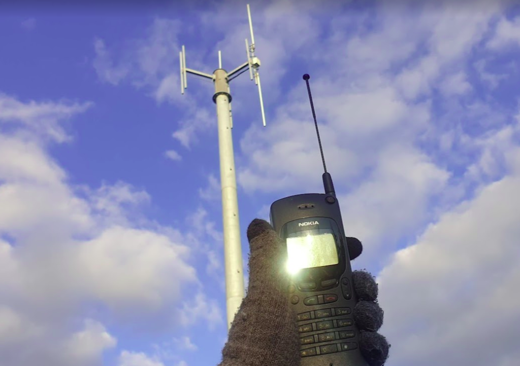
Early mobile phone networks used Vertical Polarization.
This means they used an flagpole like antenna that is vertically oriented (Omnidirectional antenna) on the base-station sites.
Oldschool mobile phones also had a little pop out omnidirectional antenna, which when you held the phone to your ear, would orient the antenna vertically.
This matches with the antenna on the base station, and away we go. You still sometimes see vertical polarization in use on base-station sites in low density areas, or small cells.
Vertically polarized mobile phone antenna, which is oriented vertically, like on the base station behind it.
Increasing subscriber demand meant that operators needed more capacity in the network, but spectrum is expensive. As we just saw a mismatch in polarization can lead to a huge reduction in power, and maybe we can use that to our advantage…
Shannon-Hartley Theorem
But first, we need to do some maths…
Stick with me, this won’t be that hard to understand I promise.
There are two factors that influence the capacity of a network, the Bandwidth of the Channel and the Signal-to-Noise Ratio.
So let’s look at what each of these terms mean.
Bandwidth
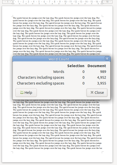
Bandwidth is the information carrying capacity. A one-page sheet of A4 at 12 point font, has a set bandwidth. There’s only so much text you can fit on one A4 sheet at that font size.
A4 Sheet, 12 point font, has 989 words.
We can increase the bandwidth two ways:
Option 1 to Increase Bandwidth: Get a larger transmission medium. Changing the size of the medium we’re working with, we can increase how much data we can transfer.
For this example we could get a bigger sheet of paper, for example an A3 sheet, or a billboard, will give us a lot more bandwidth (content carrying capability) than our sheet of A4.
Changing from an A4 sheet to an A3 sheet, increases the number of characters we can store on the page (Slightly more than doubling the bandwidth).
Option 2 to Increase Bandwidth: Use more efficient encoding As well as changing the size of the medium we are using, we can change how we store the data on the paper, for example, shrinking the font size to get more text in the same area, which also the bandwidth.
In communications networks this is also true: Bandwidth is determined by how much spectrum we have to work with (For example 10Mhz), and how we encode the data on that spectrum, ie morse-code, Binary-Phase-Shift-Keying or 16-QAM. Each of the different encoding schemes have different levels of bandwidth for the same amount of spectrum used, and we’ll cover those in more detail in the future.
So now we’ve covered increasing the bandwidth, now let’s talk about the other factor:
Signal-to-Noise Ratio
Signal-to-NoiseRatio (SNR) is the ratio of good signal, to the background noise.
On the train my headphones on block out most of the other sounds. In this scenario, the signal (the podcast I’m listening to on the headphones) is quite high, compared to the noise (unwanted sounds of other people on the train), so I have a good Signal-to-Noise ratio.
When we talk about the Signal-to-Noise Ratio, we’re talking about the ratio of the signal we want (podcast) to the noise (signal we don’t want).
When I’m on the train if 90% of what I hear is the podcast I’m listening to (the “signal”) and 10% is random background sounds (the “noise”) then my signal-to-noise-ratio is really good (high).
Capacity and SNR
Let’s continue with the listening to a podcast analogy.
The average human talks about 150 words per minute. So let’s imagine I’m listening to a podcast at 150 words per minute.
If I’m listening in an anechoic chamber, then I’ll be able to hear everything that’s being said, so my bandwidth will 150 words per minute. As there is no background noise, my capacity will also be 150 words per minute.
But if I leave an anechoic chamber (much as I love spending time in anechoic chambers), and go back on the train, I won’t hear the full 150 words per minute (bandwidth) due to the noise on the train drowning out some of the signal (podcast).
The Shannon-Hartley Theorem, states that the capacity is equal to the bandwidth multiplied by the signal to noise ratio.
So on the train hearing 90% of what’s said on the podcast, 10% drowned out, means my signal-to-noise ratio is 0.9 (pretty good).
So according to Shannon-Hartley Theorem the capacity of me listening to a podcast on the train (150 words per minute of bandwidth multiplied by 0.9 Signal-to-Noise Ratio) would give me 135 words per minute of capacity.
Claude Shannon, of 1/2 of the Shannon-Hartley Theorem, with an electromechanical mouse maze.
How this applies to RF Networks
In an RF context, our Bandwidth has a fixed information carrying capacity, for example on LTE, with a 5Mhz wide channel using 16QAM has 12.5Mbps of bandwidth available.
In a simple system, we have two levers we can pull to increase the bandwidth:
Increasing the size of the channel – If we went from a 5Mhz wide channel to a 20Mhz channel, this would give us 4x the available Bandwidth (Actually slightly more in LTE, but whatever)
Changing the encoding to cram more data on the same a size channel (From 16QAM to 64QAM would also give us 4x the available Bandwidth).
As we’ll see later in this post, there are some extra tricks (MIMO and Diversity) that we’ll look at later in this post, to increase the bandwidth of the system.
Our Signal-To-Noise (SNR) is constantly variable with a gazillion things that can influence the result. Some of the key factors that impact the SNR are the distance from the transmitter to the receiver and anything blocking the path between them (trees, buildings, mountains, etc), but there’s so many other factors that go into this. From atmospheric conditions, flat surfaces the signal can reflect off leading to multipath noise, other nearby transmitters, etc, can all influence our SNR.
Our capacity is equal to our Bandwidth multiplied by the Signal-to-Noise ratio.
Shannon-Hartley Theorem (ish)
As a goal we want capacity, and in an ideal world, our capacity would be equal to our bandwidth, but all that noise sneaks in and reduces our available capacity, based on the current SNR value.
So now we want to get more capacity out of the network, because everyone always wants to add capacity to networks.
One trick that we can use it to use multiple antennas with different polarization.
If our transmitter sends the same signal data out multiple antennas, with some clever processing on the transmitter and the receiver, we use this to maximize the received SNR. This is called Transmit Diversity and Receive Diversity and it’s a form of black magic.
The Transmitter uses feedback from the receiver to determine what the channel conditions are like, and then before transmitting the next block of data, compensates for the channel conditions experienced by the receiver, this increases the SNR and allows for higher MCS / encoding schemes, which in turns means higher throughput.
You’ll notice on most Antennas in the wild today you’ve got at least two ports for each frequency, which are + and -, which are the two polarizations.
Modern mobile networks use ±45° slant polarization (aka X Polarization), which works better in the orientations end users hold their phones in.
These two polarizations, each connected to a distinct transmit/receive path on the phone (UE) end and on the base station end, allows multiple data streams to be sent at the same time (spatial multiplexing, the foundation for MIMO) which enables higher throughput or can be configured enable redundancy in the transmission to better pick up weak signals (Diversity).
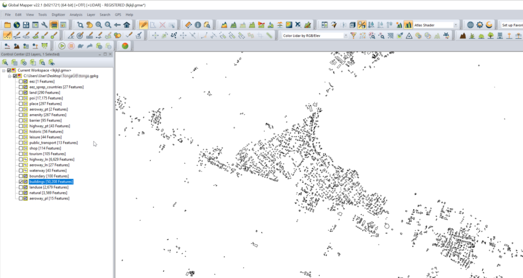
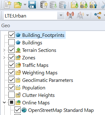
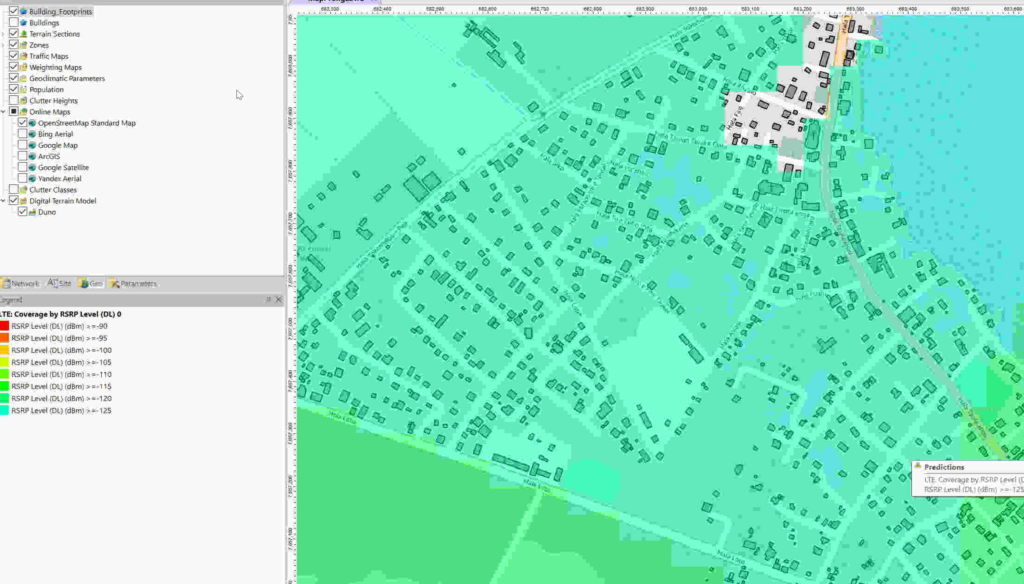
Having building footprints inside Atoll is super-duper valuable, this means you can calculate your percentage of homes / buildings covered, after all geographic coverage and population coverage are two very different things.
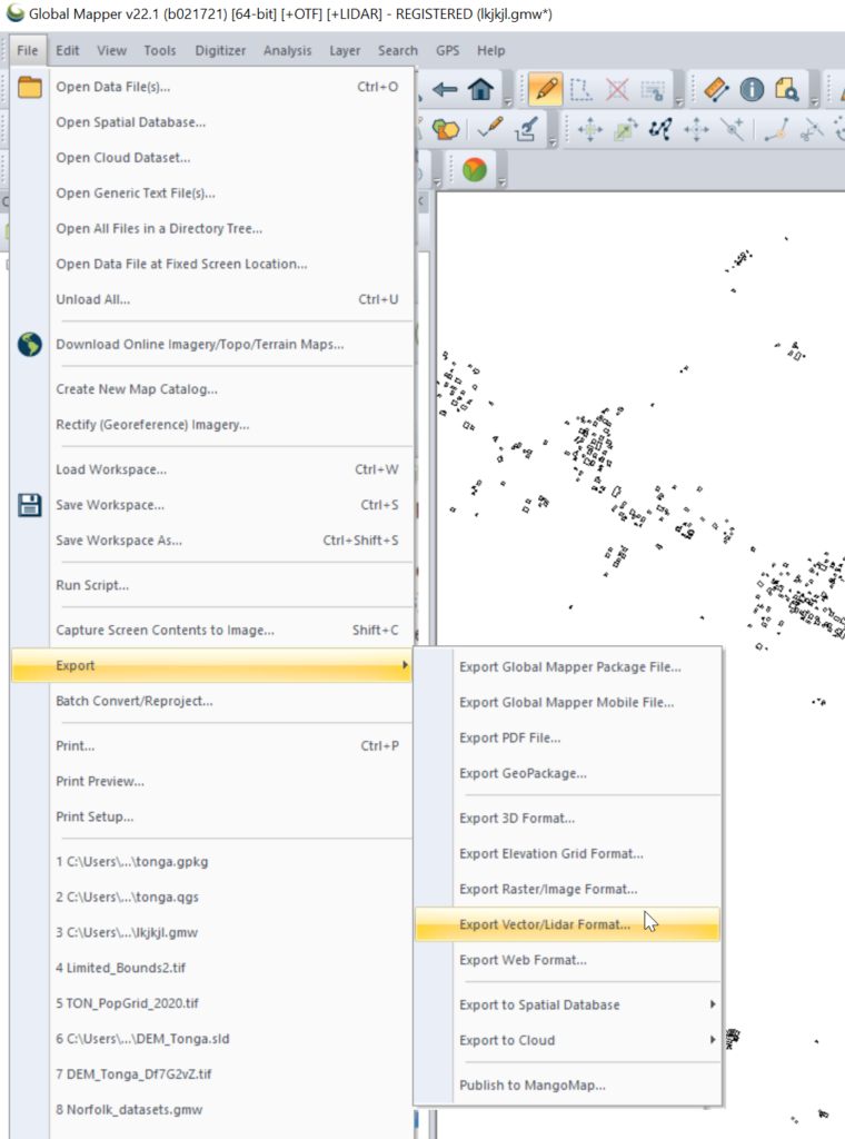
Once you’ve got the export, we’ll load the .gpkg file (or files) into GlobalMapper
Select one layer at a time that you want to export into Atoll. (This also works for roads, geographic boundaries, POIs, etc)
Export the selected layer from Export -> Export Vector / Lidar Format
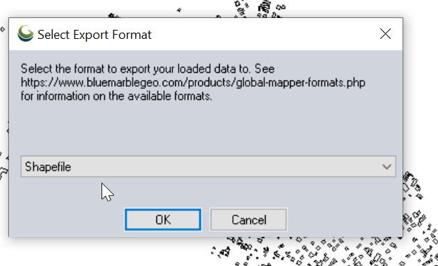
Set output type to “Shapefile”
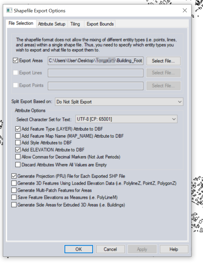
Set output filename in “Export Areas” (This will be the output file). If you want to limit the export to a given area you can do that in Export Bounds.
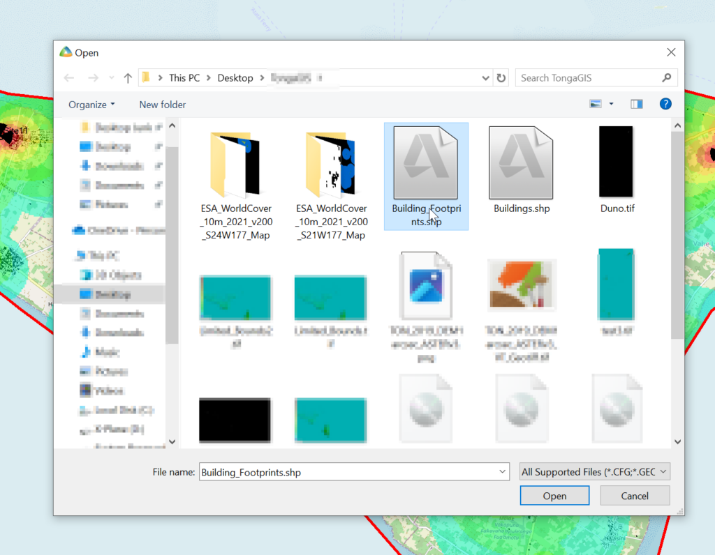
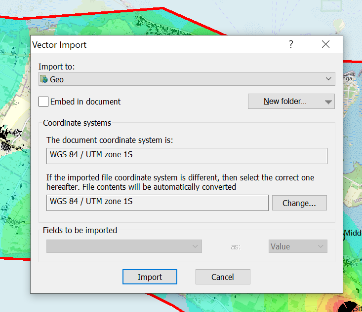
Now we can import this data into Atoll.
File -> Import
Select the exported Shapefile we just created.
Set the projection and import
Bingo now we’ve got our building footprints,
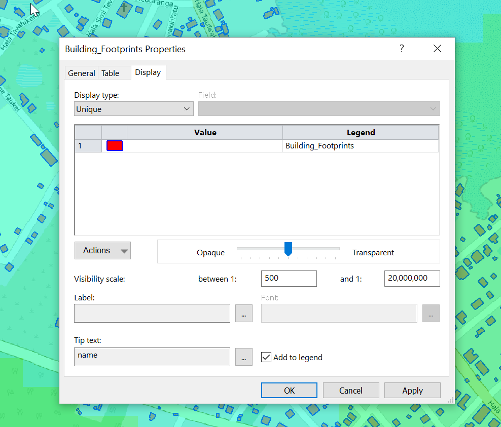
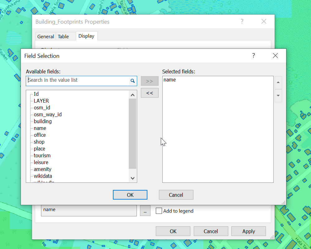
We can change the style of the layer and the labels as needed.
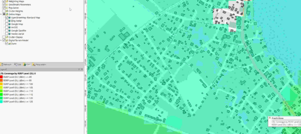
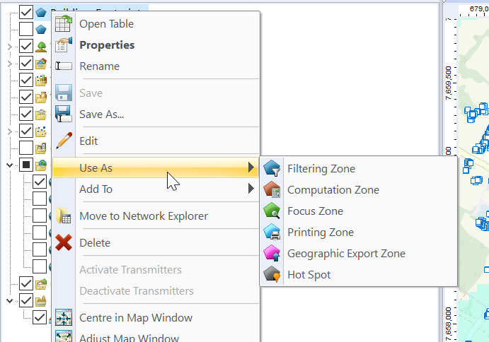
Now we can use the buildings as the Focus Zone / Compute Zone and then run reports and predictions based on those areas.
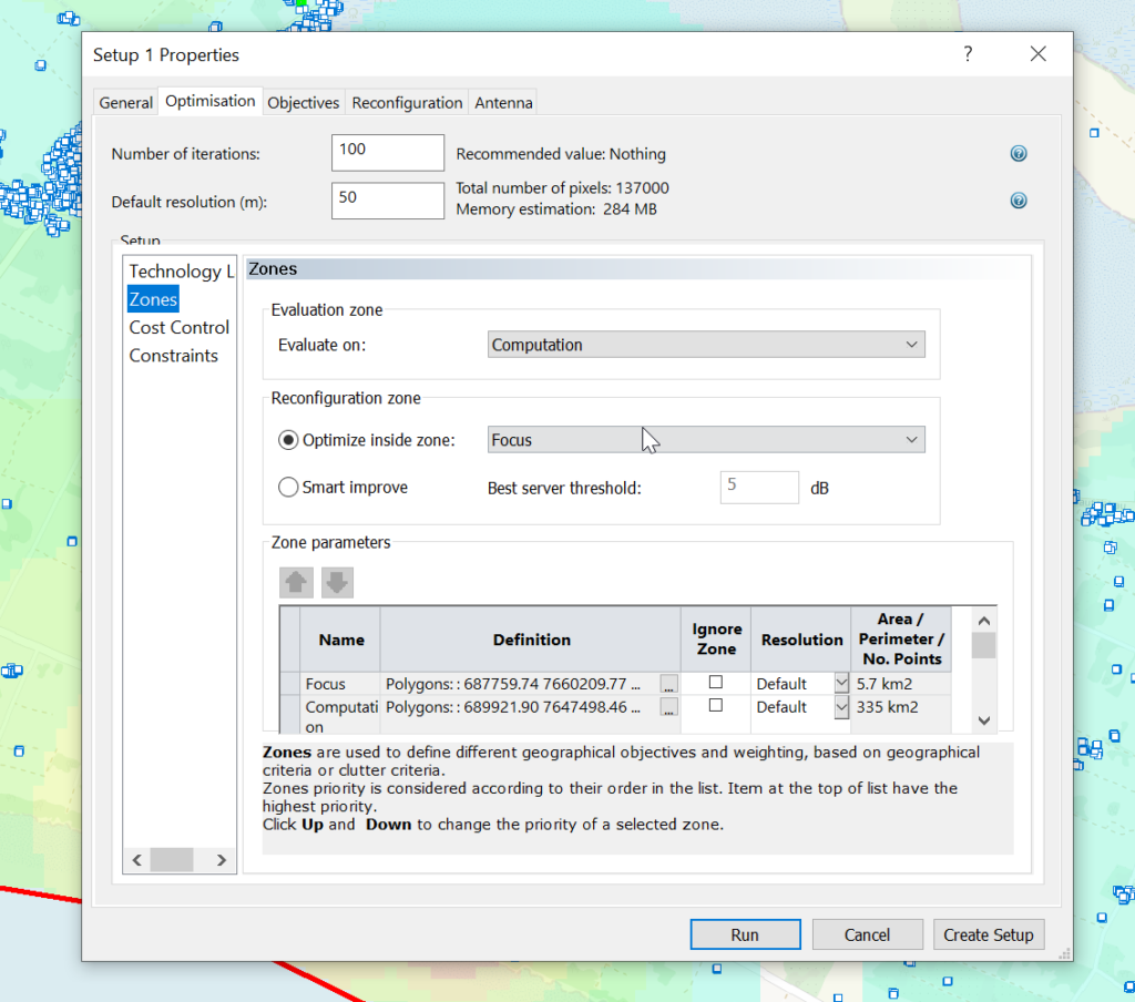
For example I can run Automatic Cell Planning with the building layers as the Focus zones, to optimize azimuths, tilts and powers to provide coverage to where people live, not just vacant land.
Clutter data describes real world things on the planet’s surface that attenuate signals, for example trees, shrubs, buildings, bodies of water, etc, etc. There’s also different types of trees, some types of trees attenuate signals more than others, different types of buildings are the same.
Getting clutter data used to be crazy expensive, and done on a per country or even per region basis, until the European Space Agency dropped a global dataset free of charge for anyone to use, that covered the entire planet in a single source of data.
So we can use this inside Forsk Atoll for making our predictions.
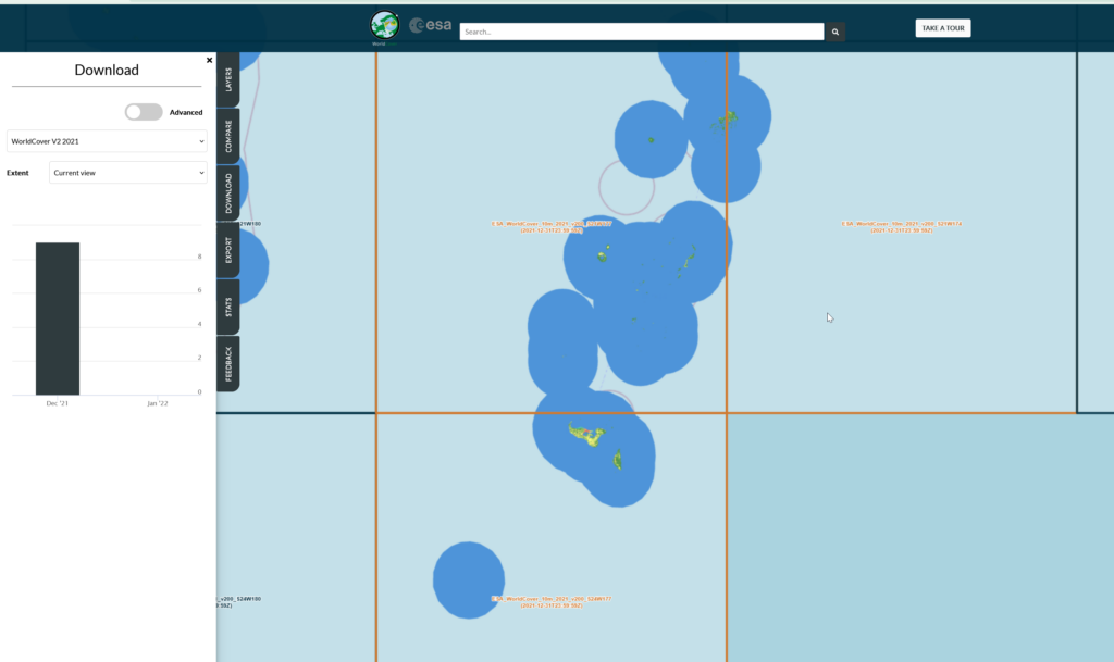
First things first we’ll need to create an account with the ESA (This is not where they take astronaut applications unfortunately, it just gives you access to the datasets).
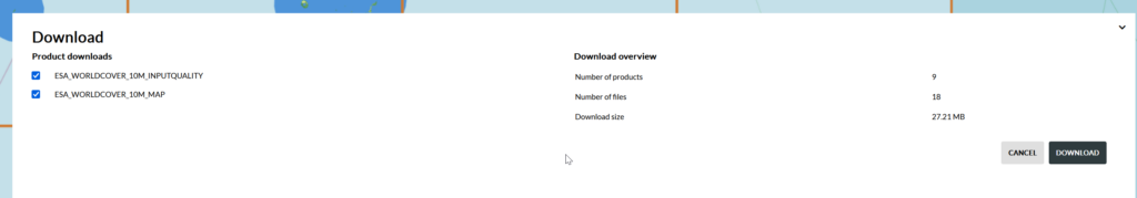
Then you can select the areas (tiles) you want to download after clicking the “Download” tab on the right.
We get a confirmation of the tiles we’re download and we’ll get a ZIP file containing the data.
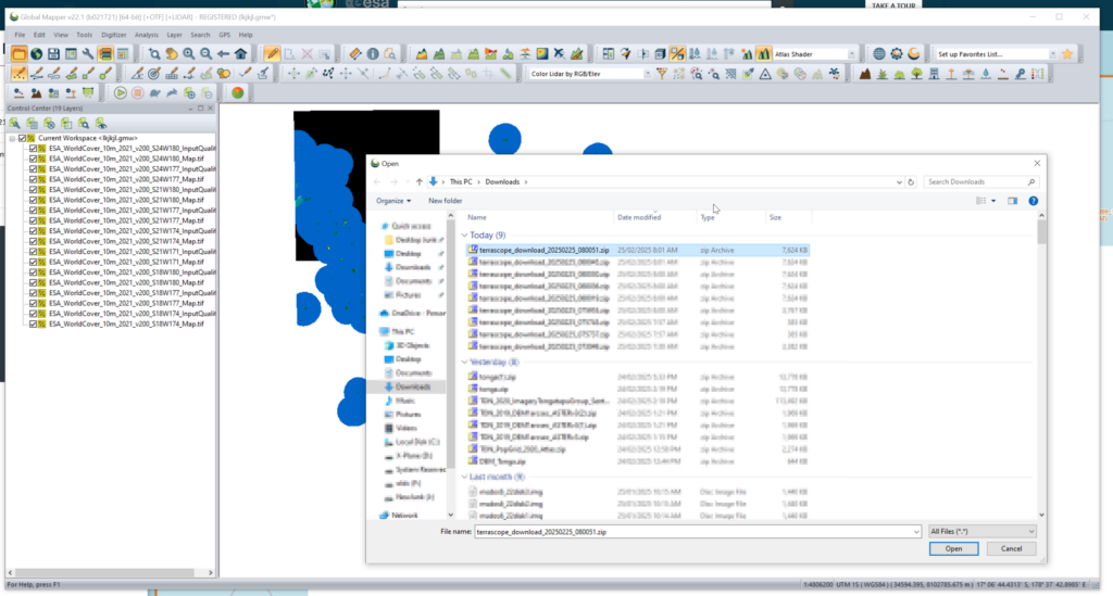
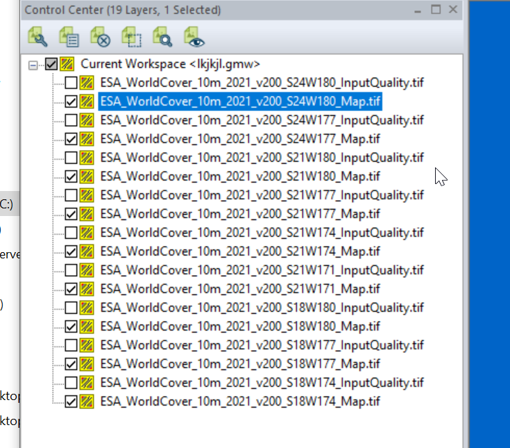
We can load the whole ZIP file (Without needing to extract anything) into GlobalMapper which loads all the layers.
I found the _Map.tif files the highest resolution, so I’m only exporting these.
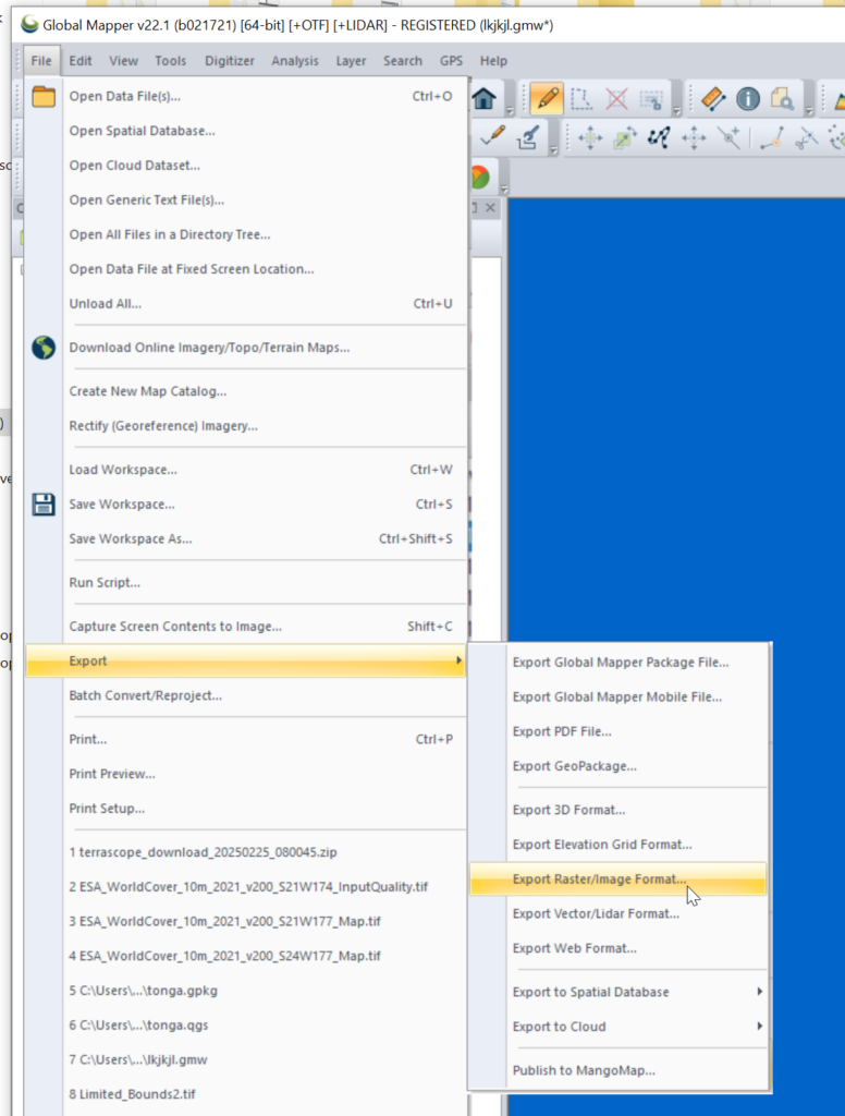
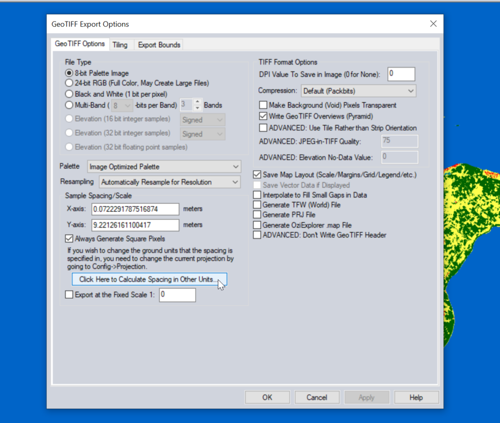
Then we need to export the data to GeoTiff for use in Atoll (The specific GeoTiff format ESA produces them in is not compatible with Atoll hence the need to convert), so we export the layers as Raster / Image format.
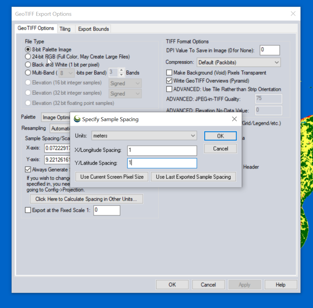
Atoll requires square pixels, and we need them in meters, so we select “Calculate Spacing in Other Units”.
Then set the spacing to meters (I use 1m to match everything else, but the data is actually only 10m accurate, so you could set this to 10m).
You probably want to set the Export Bounds to just the areas you’re interested in, otherwise the data gets really big, really quickly and takes forever to crunch.
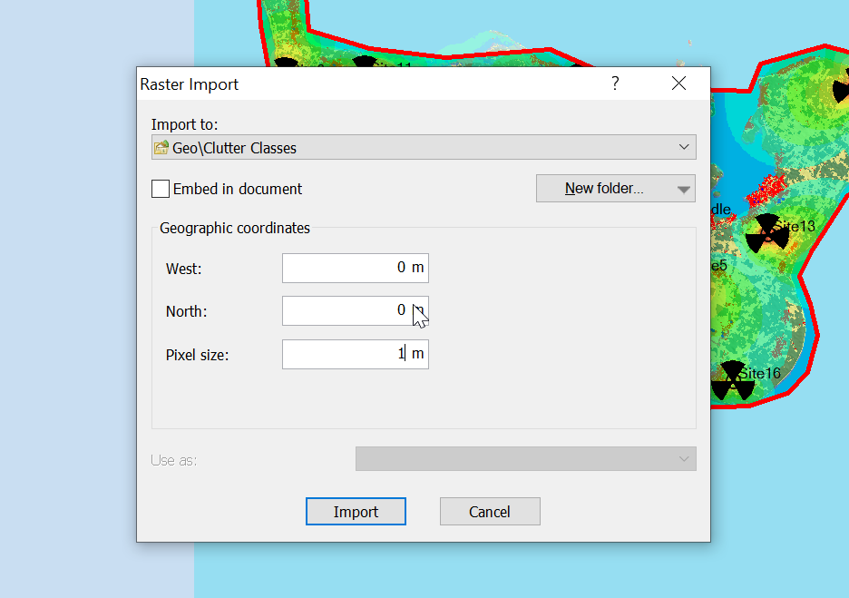
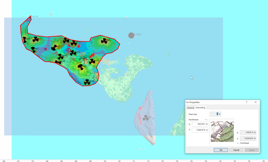
Now for the fancy part, we need to import it into Atoll.
When we import the data we import it as Raster data (Clutter Classes) with a pixel size of 1m.
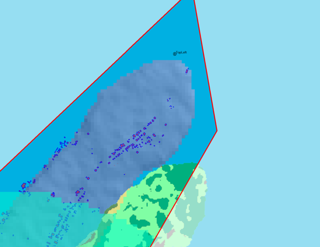
Alas when we exported the data we’ve lost the positioning information, so while we’ve got the clutter data, it’s just there somewhere on the planet, which with the planet being the size it is, is probably not where you need it.
So I cheat, I start put putting the West and North values to match the values from a Cell Site I’ve already got on the map (I put one in the top left and bottom right corners of the map) and use that as the initial value.
Then – and stick with me, this is very technical – I mess with the values until the maps line up into the correct position. Increase X, decrease Y, dialing it it in until the clutter map lines up with the other maps I’ve got.
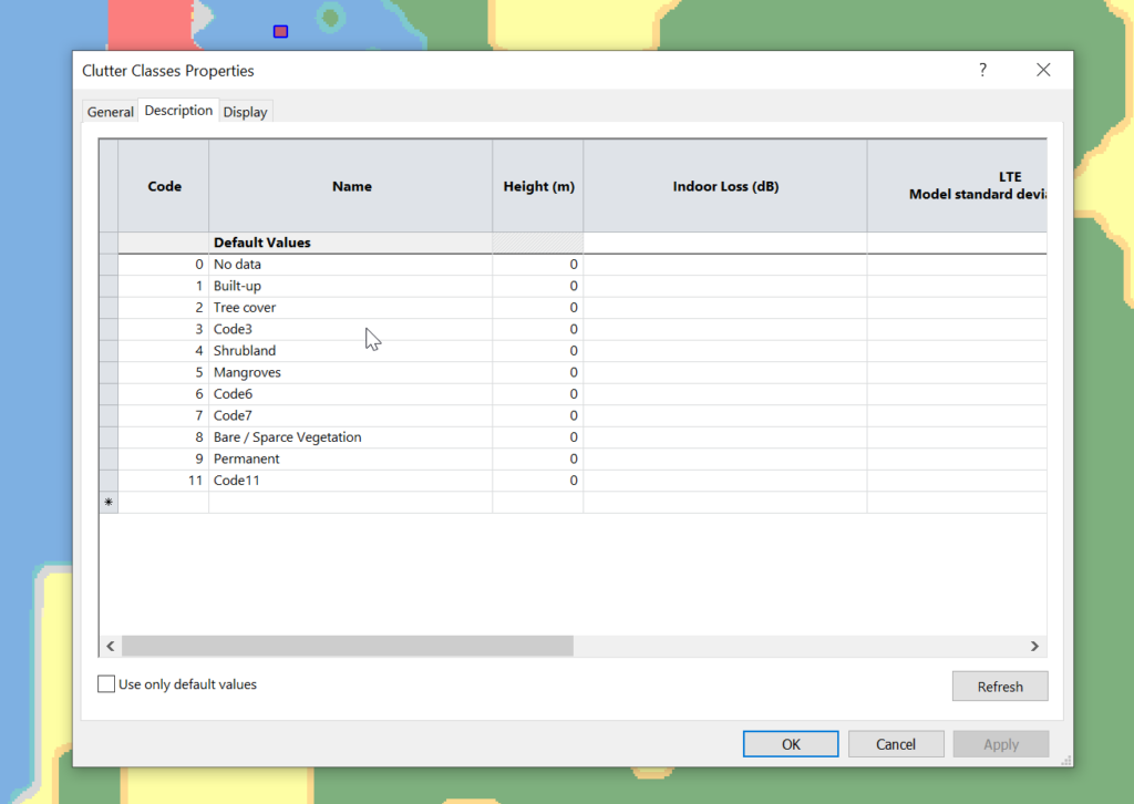
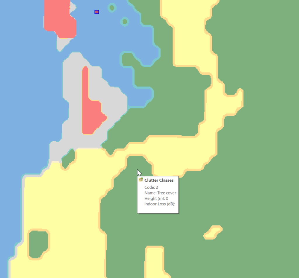
Right, now we’ve got the data but we don’t have any values.
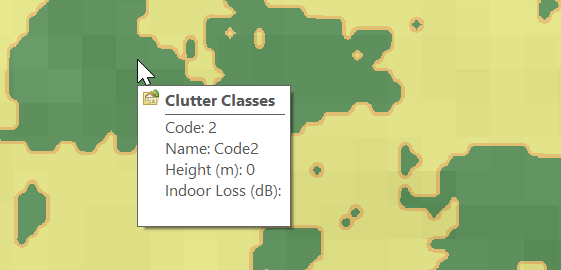
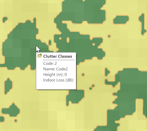
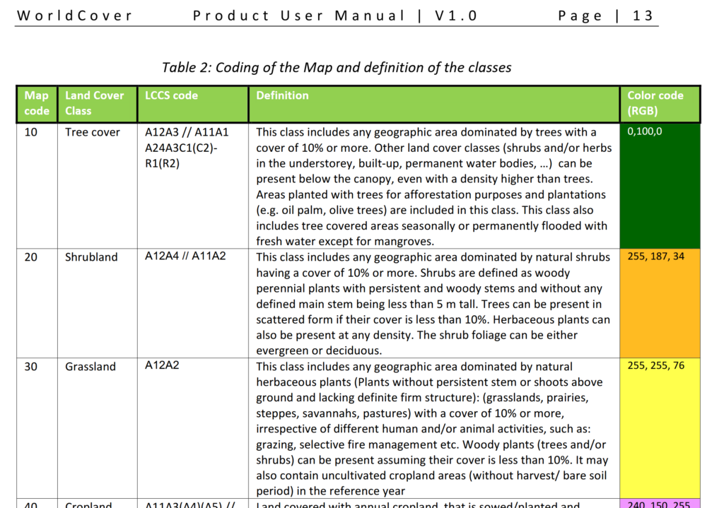
Each color represents a clutter class, but we haven’t set any actual height or losses for that material.
Alas the Map Code does not match with the table in the manual, but the colours do, here’s what mine map to:
Which means when hovering over a layer of clutter I can see the type:
Next we need to populate the heights, indoor and outdoor losses for that given clutter. This is a little more tricky as it’s going to vary geography to geography, but there’s indicative loss numbers available online pretty easily.
Once you’ve got that plugged in you can run your predictions and off you go!
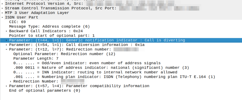
Had an interesting fault come across my desk the other day; calls were failing when the called party (an SSP we talk to via SS7/ISUP) had an exchange based call forward in place.
We’re a SIP based network, but we do talk some SS7/ISUP on the edges, and it was important that we handled this correctly.
I could see in the Address Complete Message (ACM) sent back to our network that there was redirection information here:
We would see the B party SSP release the call as soon as it sent this.
This made me wonder if we, as the originating network, were supposed to redirect to the new B party and send a new Initial Address Message?
After a lot of digging in the ITU Q.7xx docs (I’m not where near as fast at finding information in specs written prior to my birth, than I am with the 3GPP specs) I found my answer – These headers are informational only, the B party SSP is meant to re-target the message, and send us an Alerting or Answer message when it’s done so.
CAMEL is primarily focused on charging for Voice & SMS services, as data generally uses Diameter, so it’s voice and SMS we’ll focus on.
CAMEL is spoken between the MSC (gsmSSF) and the OCS (gsmSCF).
Basic Call State Model
CAMEL is closely related to the Intelligent Network stuff on the 1980s, and steals a lot of it’s ideas from there, unfortunately if you’re to read the CAMEL standard it also implies you were involved in IN stuff and had been born at that point, alas I was neither.
So the key to understanding CAMEL is the Basic Call State Model (BCSM) which is a model of all the different states a call can be in, such as ringing, answered, abandoned, call failed, etc, etc.
Over CAMEL, our OCS can be told by the MSC when a certain event happens; the MSC can tell the OCS, that the call has changed state. For example a BCSM event might indicate the call has hung up, is ringing, cancelled, etc.
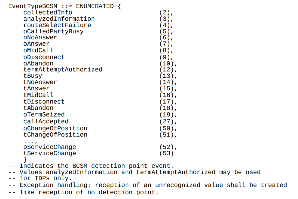
Below is the list of all the valid BCSM states:
List of BCSM states for events
Basic MO Call with CAMEL
Our subscriber makes an outbound call.
Based on the data the MSC has in it from the HLR, it knows that we should use CAMEL for this call, and it has the SCCP Address of the OCS (gsmSCF) it needs to send the CAMEL messages to.
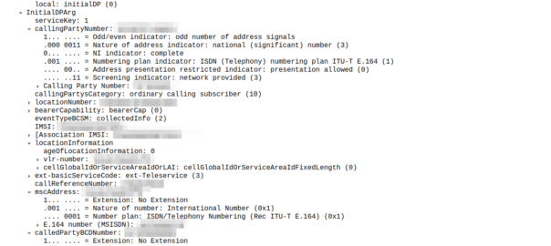
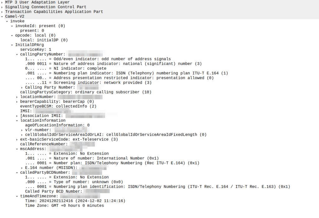
So the MSC sends an InitialDP message to the OCS (via it’s Global Title Address) to Authorize the call that the user is trying to make.
This is like any other Authorization step for an OCS, which allows the OCS to authorize the call by checking the subscriber is valid, check if they’re allowed to call that destination and they’ve got the balance to do so, etc.
initialDP message from an MSC to an OCS
The initialDP (Initial Detection Point) is telling our OCS all about the call event that’s being requested, who’s calling, what number they’ve dialed, where they are in the network (of note especially if they’re roaming), etc, etc.
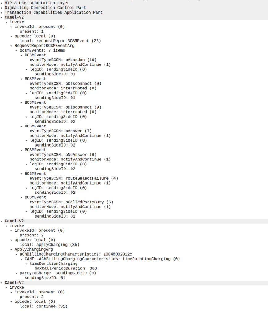
Generally the OCS also uses this message as a chance to subscribe to BCSM Events using RequestReportBCSMEventArg so the OCS will get notified by the MSC when the state of the call changes. This means the MSC will tell us when the state of the call changes; events like the call getting answered, disconnected, etc. This is critical so we know when the call gets answered and hung-up, so we can charge correctly.
In the below example, as well as sending the Continue and RequestReportBCSMEventArg the OCS is also setting the ChargingArgs for this call, so the MSC knows who to charge (the caller) set via sendingSide and that the MSC must send an Apply Charging Report (ACR) messages every 300 units (1 unit = 100 ms, so a value of 300 = 300 x 100 milliseconds = 30 seconds) so the OCS keeps track of what’s going on.
continue sent by the OCS to the MSC, also including reportBCSMEvent and applyCharging messages
Or in a slightly less appropriate analogy but easier to understand for SIP folks, the InitialDP is sent for INVITE and the 180 RINGING is sent once the continue message is received.
Call is Answered
So at this stage our call can start to ring.
As we’ve subscribed to BCSM events in our last message, the MSC is going to tell us when the call gets answered or the call times out, is abandoned or the sun burns out.
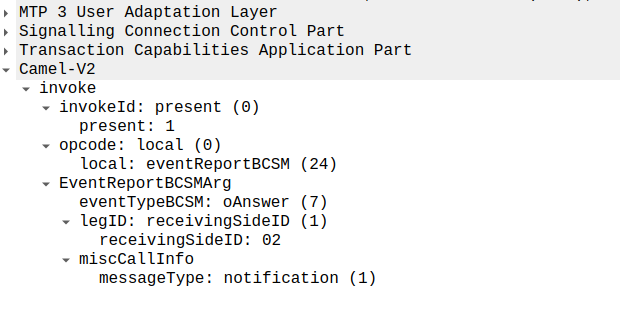
The MSC provides this info a eventReportBCSM, which is very simple and just tells us the event that’s been triggered, in the example below, the call was answered.
eventReportBCSM from MSC to OCS
These eventReportBCSM are informational from the MSC to the OCS, so the OCS doesn’t need to send anything back, but the OCS does need to mark the call as answered so it can start timing the call.
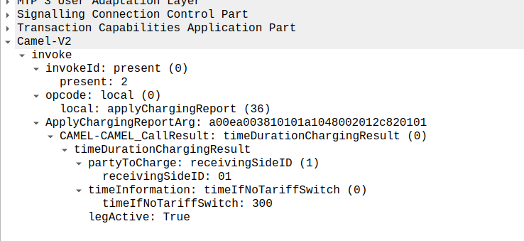
At this stage, the call is connected and our two parties are talking, but our MSC has been told it needs to send us applyChargingReports every 30 seconds (due to the value of 300 in maxCallPeriodDuration) after the call was connected, so the MSC sends the OCS it’s first applyChargingReport 30 seconds after the call was answered:
applyChargingReport sent by the MSC to the OCS every reporting period
We can calculate the duration of the call so far based on the time of the eventReportBCSM, then the OCS must make a decision of if it should allow the call to continue or not.
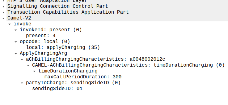
For simplicity’s sake, let’s imagine we’re still got a balance in the OCS and the OCS wants the call to continue, the OCS send back an applyCharging message to the MSC in response, and includes the current allowed maxCallPeriodDuration, keeping in mind the value is x100 and in nanoseconds (so this is 30 seconds).
applyCharging from the OCS back to the MSC
Perfect, our call is good to go for another 30 more seconds, son in 30 seconds we’ll get another ACR messages from MSC to the OCS to keep it abreast of what’s going on.
Now one of two things is going to happen, either subscriber is going to burn through all of their minutes, and get their call cutoff, or the call will end while they’ve still got balance, let’s look at both scenarios.
Normal Hangup Scenario
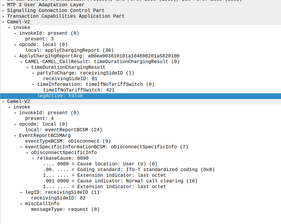
When the call ends, we get an applyChargingReport from the MSC to the OCS.
As we’ve subscribed to reportBCSMEvent we get both the applyChargingReport with legActive: False` so we know the call has hungup, and we’ve got an event report to tell us more about the event, in this case a hangup from the Originating Side.
reportBCSMEvent and applyChargingReport Sent by the MSC to the OCS to indicate the call has ended, note the legActive flag is now false
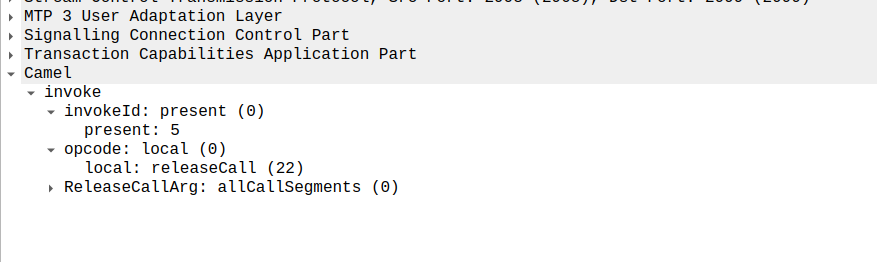
Lastly the OCS confirms by sending a releaseCall to the MSC, to indicate all legs should now terminate.
releaseCall Sent by OCS to MSC at the very end
So that’s it!
Obviously there are other flows, such as running out of balance mid-call, rejecting a call, SMS and PBX / VPN services that rely on CAMEL, but hopefully you now understand the basics of how CAMEL based charging looks and works.
If you’re looking for a CAMEL capable OCS or a CAMEL to Diameter or API gateway, get in touch!
When Dickens wrote of Doctor Manette in the 1859, I doubt his intention was to write about the repeating history of RAN fronthaul standards – but I can’t really say for sure.
Setting the Scene
Our story starts with introducing CPRI (Common Public Radio Interface) interface, having been imprisoned in the Bastille of vendor lock in for the better part of twenty years.
Think of CPRI is less of a hard interoperable standard and more like how the Italian and French languages are both derived from Latin; it doesn’t mean that the two languages are the same, but they’ve got the same root and may share some common words and structures.
In practice this means that taking an Ericsson Radio and plugging it into a Huawei Baseband simply won’t work – With CPRI you must use the same vendor for the Baseband and the Radios.
“Nuts to this” the industry said after being stuck locked between the same radios and baseband for years; we should create a standard so we can mix and match between radio vendors, and even standardize some other stuff that’s been bothering us, so we’ll have a happy world of interoperability.
A world with interoperable fronthaul
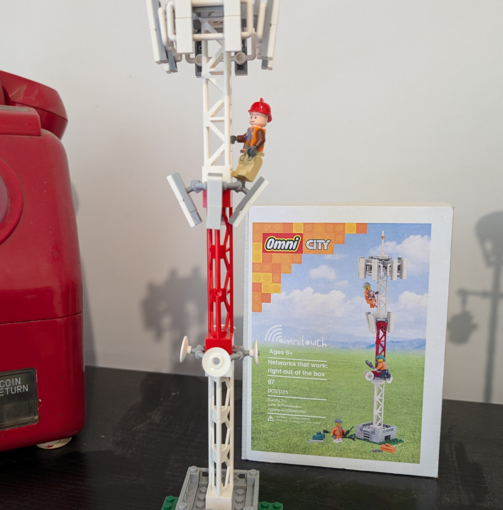
With kit created that followed this standard, we’d be able to take components from vendor A, B & C, and fit them together like Lego, saving you some money along the way and giving you’ve got a working solution made of “best of breed” components, where everything is interoperable.
Omnitouch Lego base stations, which also fit together like Lego – Part of the Omnitouch Network Services “swag” from 2024
So the industry created a group to chart a path for a better tomorrow by standardizing these interfaces.
The group had many industry heavyweights like Nokia, NEC, LG, ZTE and Samsung joining.
The key benefits espoused on their website:
An open market will substantially reduce the development effort and costs that have been traditionally associated with creating new base station product ranges. The availability of off-the-shelf base station modules will enable manufacturers to focus their development efforts on creating further added value within the base station, encouraging greater innovation and more cost-effective products. Furthermore, as product development cycles will be reduced, new base station functions will become available on the market more quickly.
Mission statement of the group
In addition to being able to mix and match radios and basebands from different vendors, the group defined standards for centralized baseband, and interoperable standards, to allow a multi-vendor ecosystem to flourish.
And here’s the plot twist – The text above, was not written about OpenRAN, and it was not written about the benefits of eCPRI.
It was written about Open Base Station Architecture Initiative (OBSAI) and it was written 22 years ago.
*record screech sound*
Standards War you’ve never heard of: OBSAI vs CPRI
When OBSAI was defined it was not without competition; there was another competing fronthaul standard; that’s right, the mustache twirling lowlife from earlier in the story – CPRI.
Supported by Huawei, Nortel, NEC & Ericsson (among others), CPRI took a “gentle parenting” approach to the standards world, in contrast to OBSAI. Instead of telling all the vendors to agree on an interoperable front haul standard, CPRI just encouraged everyone to implement what their heart told them and what felt right to them.
As it happened, the industry favored the CPRI approach.
If a vendor wanted to add a new “word” in their CPRI “language” to add a new feature, they just went ahead and added it – It didn’t require anyone else to agree with them or changes to a common standard used by the industry, vendors could talk to the kit they made how they wanted.
CPRI has been the defacto non-standard used by all the big kit vendors for the past ~10 years.
The Death of OBSAI & the Birth of OpenRAN’s eCPRI
Why haven’t you heard of OBSAI? Why didn’t the OBSAI standard just serve as the basis for eCPRI – After all the last OBSAI release was less than 5 years before TIP started working on eCPRI publicly.
Is no more. It has ceased to be.
Did a schism over “uplink performance improvement” options lead to “irreconcilable differences” between parties leading to the breakup of the OBSAI group?
Nope.
Customers (MNOs) didn’t buy OBSAI based equipment in measurably larger quantities than CPRI kit. That’s it.
This meant the vendors invested less in paying teams to further develop the standards, the OBSAI group met less frequently, and in the end, member vendors didn’t bother adding support for OBSAI to new equipment and just used the easier and more flexible CPRI option instead.
At some point someone just stopped paying for the domain renewal and that was it, OBSAI was no more.
This is how the standards body ends, not with a bang, but with a whimper.
T.S. Elliot’s writings on the death of obsai
Those who do not learn from history…
The goals of the OBSAI Group and OpenRAN working groups are almost identical, so what lessons did Marconi, Motorola and Alcatel learn as members of OBSAI that other vendors could learn about OpenRAN strategy?
There are no mentions of OBSAI in any of the information published by OpenRAN advocates, and I’m wondering if folks aren’t aware that history tends to repeat and are ignorant to what came before it, or they’re just not learning lessons from the past?
So what can the OpenRAN industry learn from OBSAI?
Being a nerd, I started detailing the technical challenges, but that’s all window dressing; The biggest hurdle facing CPRI vs eCPRI are the same challenges OBSAI vs CPRI faced a decade prior:
To be relevant, OpenRAN kit has to be demonstrably better than what we have today AND provide a tangible cost saving.
OBSAI failed at achieving this, and so failed to meet it’s other more noble goals.
[At the time of writing this at least] I’d contend that neither of those two criteria have been met by OpenRAN.
What does the future hold for OpenRAN?
Looking into the crystal ball, will OpenRAN and eCPRI go the way of OBSAI, or will someone keep the OpenRAN dream alive?
Today, we’re still seeing the MNOs continue to provide tokenistic investment in OpenRAN. But being a cynic, I’d say the MNOs are feigning interest in OpenRAN products because it’s advantageous for them to do so.
The threat of OpenRAN has proven to be a great stick to beat the traditional vendors with to force them to lower their prices.
Think about the $14 billion USD Ericsson deal with AT&T, if chucking a few million at OpenRAN pilots / trials lead to AT&T getting even a 0.1% reduction in what they’re paying Ericsson, then the numbers would have worked out well in AT&Ts favor.
From the MNOs perspective, the cost to throw the odd pilot or trial to a hungry OpenRAN vendor to keep them on the hook is negligible, but the threat of OpenRAN provides leverage and bargaining power every time it’s contract renewal time with the big RAN vendors.
Already we’ve seen all the traditional RAN vendors move to neutralize this threat by introducing “OpenRAN compatible” equipment and talking up their commitment to openness.
This move by the RAN vendors takes this sting out of the OpenRAN threat, and means MNOs won’t have much reason to continue supporting OpenRAN.
This leaves the remaining OpenRAN vendors like Miss Havisham, forever waiting in their proverbial wedding dresses, having being left at the altar.
Okay, I’m mixing my Dickens’ references here, but it was too good not to.
Appendix
I’ve been enjoying writing more analysis than just technical content, let me know if this is something you’re interested in seeing more of.
I’ve been involved in two big OpenRAN integration projects, both of which went poorly and probably tainted my perspective. Enough time has passed to probably write up how it all went with the vendor names removed, but that’s a post for another time!
This is the next post in my series on SS7, and today we’re taking a look at SCCP the Signalling Connection Control Part (SCCP).
High Level
Global Title uses the routing features from SCCP, which is another layer on top of MTP3.
SCCP allows us to route on more than just point code, instead we can route based on two new fields, Subsystem Number and Global Title.
Subsystem Number is the type of system we are looking to reach, ie an HLR, MSC, CAMEL Gateway, etc.
The Global Title generally looks like an E.164 formatted phone number, and often it is just that.
Somewhere along the chain (typically at the end of it) an STP somewhere needs to perform Global Title Translation to analyse the SCCP header (Subsystem Number, Point Code & Global Title) and finally turn that into a single point code to route the MTP3 message to.
The advantage of this is we are no longer just limited to routing messages based on Point Code.
This is how the international SS7 Network used for roaming is structured and addressed – All using Global Title rather than Point Codes.
The need for SCCP
For starters, after all this talk of MTP3 and Point Codes, why the need to add SCCP?
Let’s go back in time and look at the motivators…
1. Address space is finite
Point codes are great, and when we’ve spoken about them before, I’ve compared them to IPv4 address, but rather than ranging from 0.0.0.0 to 255.255.255.255 (32 bits on IPv4) international signaling point codes range from 0.0.0 to 7.255.7 (14 bits).
The problem with IPv4’s 32 bit addresses is they run out. The problem with the ITU International Signaling Point Codes is that they too, are a limited resource with only 16,383 possible ISPCs.
~700 operators worldwide each with ~100 network elements would be 70k point codes to address them all – That’s not going to fit into our 16k possible Point Codes.
Global Title fixes this, because we’re able to use E.164 phone number ranges (which are plentiful) for addressing, we’re still not at IPv6 levels of address space, but pretty hefty.
2. Service Discovery by Subsystem
Now imagine you’re a VLR looking to find an HLR. The VLR and the HLR are both connected to an STP, but how does the VLR know where to reach the HLR?
One option would be to statically set every route for the Point Code of every HLR into every possible VLR and visa-versa, but that gets messy fast.
What if the VLR could just send a request to the STP and indicate that the request needs to be routed to any HLR, and the STP takes care of finding a SS7 node capable of handling the request, much a Diameter Routing Agent routes based on Application ID.
SCCP’s “Subsystem Number” routing can handle this as we can route based on SSN.
3. Service Discovery by MSISDN
Having an SMS destined to a given MSISDN requires the SMSc to know where to route it.
Likewise an MSC wanting to call a given number.
There’s a lot of MSISDN ranges. Like a lot. Like every phone mobile number.
Having every a table on every SSP/SCP in the network know where every MSISDN range is in the world and what point code to go through to reach it is not practical.
Instead, being able to have the SCP/SSPs (like our MSC or SMSc) send all off-net traffic to an STP frees us the individual SCP/SSPs from this role; they just forward it to their connected STP.
Our STP can analyse the destination MSISDN and make these routing decisions for us, using Global Title Translation based on rules in the Global Title Table on the STP.
For example by adding each of the domestic / national MSISDN ranges/prefixes into the Global Title Table on the STP (along with the corresponding point code to route each one to), the STP can look at the destination MSISDN in the message and forward to the STP for the correct operator.
Likewise a route can match anything where the Global Title address is outside of the local country and send it to an international signaling provider.
Global title takes care of this as we can route based on a phone number.
4. Tokenistic Security
By “Hiding” network elements behind Global Titles, you don’t expose as much information about your internal network, and the only way people can “find” your network elements would be scanning through all the possible addresses in your (publicly advertised) Global Title range (wardialing is back baby!).
But the phrases “Security” and “SS7” don’t really belong together…
The SCCP Header
The SCCP header has a Called Party and a Calling Party, and this is where the magic happens.
These can be made up for any number of 3 parts:
Global Title Address
Subsystem Number
Point Code
We can route on any combination of these.
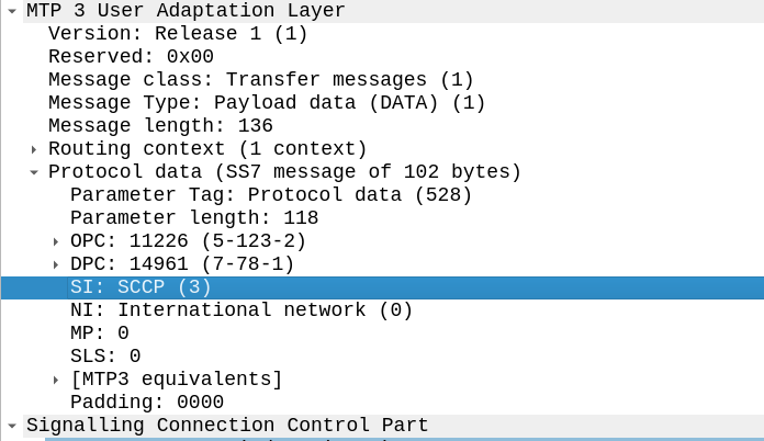
To indicate we’re using SCCP, we set the Signaling Indicator bit in the M3UA / MTP3 message to SCCP:
Great, now we can look at our SCCP header.
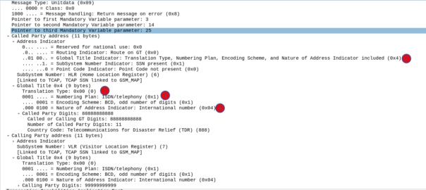
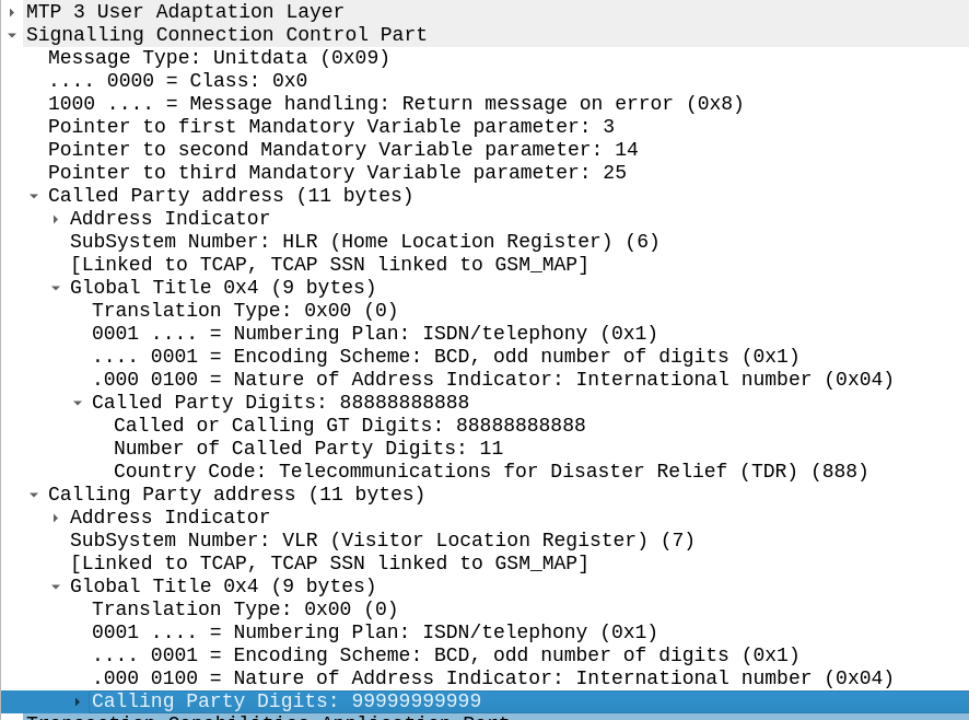
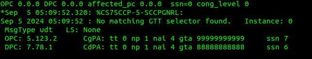
It looks like there’s a lot going on, but we can see the calling and called party (888888888 is called by 9999999999) with the Subsystem number set (888888888 is called for subsystem HLR, from 999999999 which is a VLR).
The closest TCP/IP analogy I can think of here is that of port numbers, there’s still an IP (Point code) but the port number allows us to specify multiple applications that run at a higher layer. This analogy falls down when we consider that the Point Code is generally set to that of your STP, not the final STP.
For this to work, we’ve got to have at least one Signaling Transfer Point in the flow, where we send the request to.
Somewhere (generally at the end of the chain of STPs), an STP is going to perform Global Title Translation.
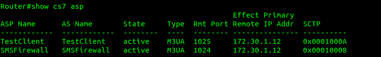
What does this look like? Well let’s have a look at my GT table for the example above, in my lab network, I’ve got two nodes attached (via M3UA but could equally be on MTP3 links), my test MAP client where I’m originating this traffic, and an SMS Firewall, I can see they’re both up here:
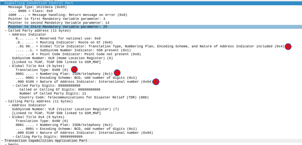
Now knowing this I need to setup my SCCP routing for Global Title. In the screenshot above, the Called Party was 888888888 with Subsystem Number 7. Inside the SCCP request, there’s a few other fields, the Translation Type we have set to 0, Global Title Indicator is 4 (route on Global Title), while Numbering Plan Indicator is 1 (ISDN) and Nature of Address Indicator is 4 (International).
So on my Cisco ITP I define a GTT Selector to target traffic with these values, Translation Type is 0, Global Title Indicator is 4, Number Plan is 1 and the Nature of Address Indicator is 4.
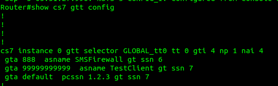
So we’d define a Global Title Translation selector like the one below to match this traffic:
But that’s only matching the group of traffic, it’s not going to match based on the actual SCCP Called Party. So now I need to define a translation for each Global Title address (Called /Calling party) or prefix I want to route, I’ve setup anything starting with 888 to route to the `SMSFirewall` ASP endpoint.
I could stop here and my request addressed to 888888888 would make it to the SMSFirewall ASP, but the response never would, like in all SS7 routing, we need to define the return route translation too, which is what I’ve done for 999999 to route to the TestClient.
Lastly I’ve added a wildcard route, this means if this STP doesn’t know how to resolve a GT address matching the rules in the top line, it’ll forward the request to the STP at point code 1.2.3 – This is how you’d do your connection to an IPX / Signaling exchange.
Debugging this can be a massive pain in the backside, but if you enable logging you can see when GT rules are not matched, like in the example below.
If your network is quiet enough, it’s sometimes easier to just make your rules based on what you observe failing to route.
So with those routes in place, when we send a request with the Global Title called party starting with 8888888 it’s routed to M3UA ASP SMSFirewall, which handles the request, and then sends the response back to the MAPClient M3UA ASP.
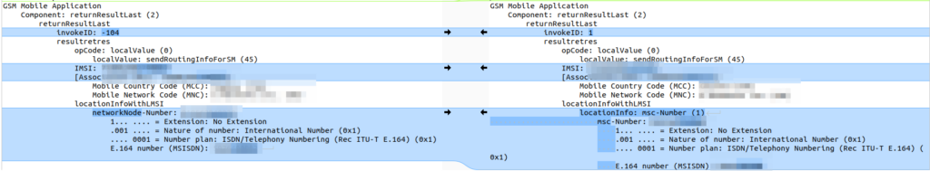
The other day I was facing an issue with our SMSc inter-working with another operator via MAP.
Our SRI-for-SM responses were relayed back to their nodes, but it was like it couldn’t parse the message.
I got some “known good” traffic to compare this against to work out what we’re doing wrong.
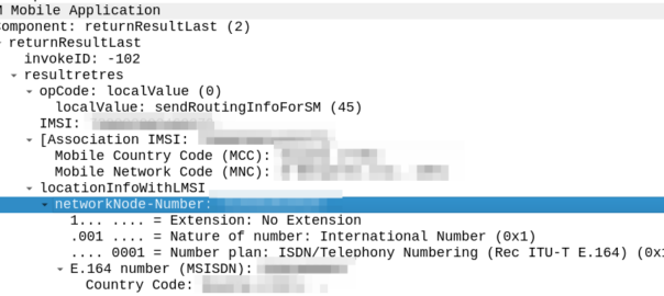
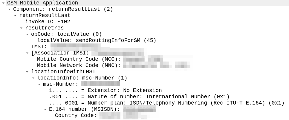
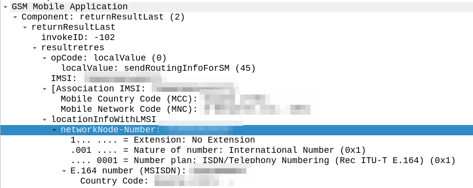
The difference in the two examples below is subtle, but it’s there – On the example on the left (failing) we are including an msc-number in the locationInfoWithLMSI field, while on the right we’ve got a “Network Node Number”.
“Okay” I thought to myself, we’re just doing something wrong with the encoding of the MAP body, so I did my usual diff trick from Wireshark:
Oddly in the raw form both these values decode the same, if I feed the values on the left into our decoder, and then encode, I get the values on the right, with the exact same hex body – and this is all ASN.1; so there’s very little room for error anyway.
So what gives? Why does Wireshark show one MAP body differently to the other, with the same hex bytes?
Well, the issue is not within my GSM MAP body and the content I include there, but rather in the TCAP layer above it, specifically the `application-context-name`.
We’re indicating support for GSM MAP v3 (0.4.0.0.1.0.20.3), while the other operator is using MAPv2 ( 0.4.0.0.1.0.20.2 ) even though their IR.21 indicates it should be GSM MAP v3.
Now our SRI-for-SM responses are based on the GSM MAP version received, rather than reported as supported, and we don’t have to deal with this for handling requests anymore.
Hello Nick, thank you for the article. What is the use of the OPc key to be derived from OP key ? Why can’t it just be a random key like Ki ?
It’s a super good question, and something I see a lot of operators get “wrong” from a security best practices perspective.
Refresher on OP vs OPc Keys
The “OP Key” is the “operator” key, and was (historically) common for an operator.
This meant all SIMs in the network had a common OP Key, and each SIM had a unique Ki/K key.
The SIM knew both, and the HSS only needed to know what the Ki was for the SIM, as they shared a common OP Key (Generally you associate an index which translates to the OP Key for that batch of SIMs but you get the idea).
But having common key material is probably not the best idea – I’m sure there was probably some reason why using a common key across all the SIMs seemed like a good option, and the K / Ki key has always been unique, so there was one unique key per SIM, but previously, OP was common.
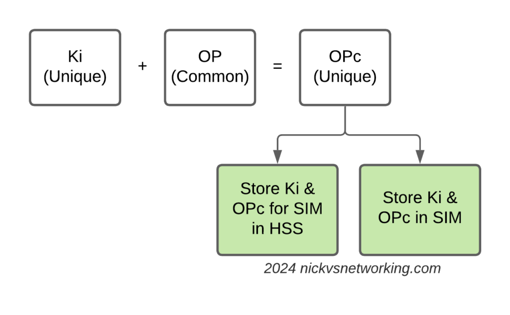
Over time, the issues with this became clear, so the OPc key was introduced. OPc is derived from mushing the K & OP key together. This means we don’t need to expose / store the original OP key in the SIM or the HSS just the derived OPc key output.
This adds additional security, if the Ki for a SIM were to be exposed along with the OP for that operator, that’s half the entropy lost. Whereas by storing the Ki and OPc you limit the blast radius if say a single SIMs data was exposed, to only the data for that particular SIM.
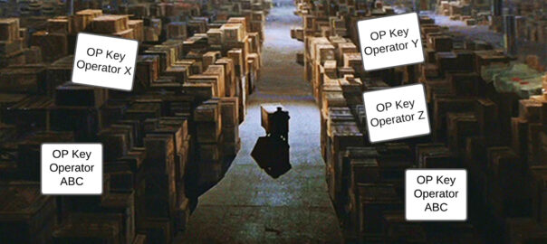
This is how most operators achieve this today; there is still a common OP Key, locked away in a vault alongside the recipe for Coca-cola and the moon landing set.
But his OP Key is no longer written to the SIMs or stored in the HSS.
Instead, during the personalization process (The bit in manufacturing where SIMs get the unique data written to them (The IMSI & keys)) a derived OPc key is written to the card itself, and to the output files the operator then loads into their HSS/HLR/AuC.
This is not my preferred method for handling key material however, today we get our SIM manufacturers to randomize the OP key for every card and then derive an OPc from that.
This means we have two unique keys for each SIM, and even if the Ki and OP were to become exposed for a SIM, there is nothing common between that SIM, and the other SIMs in the network.
Do we want our Ki to leak? No. Do we want an OP Key to leak? No. But if we’ve got unique keys for everything we minimize the blast radius if something were to happen – Just minimizes the risk.
How does one encode / interpret the value of this AVP / IE was the question I set out to answer.
TS 29.274 says:
For the encoding of this information element see 3GPP TS 32.298
TS 32.298 says:
The functional requirements for the Charging Characteristics as well as the profile and behaviour bits are further defined in normative Annex A of TS 32.251
TS 32.251 Annex A says:
The Charging Characteristics parameter consists of a string of 16 bits designated as Behaviours (B), freely defined by Operators, as shown in TS 32.298 [51]. Each bit corresponds to a specific charging behaviour which is defined on a per operator basis, configured within the PCN and pointed when bit is set to “1” value.
After a few circular references I found this is imported from 32.298.
Finally we find some solid answers hidden away in TS 132 215, under the Charging Characteristics Profile index.
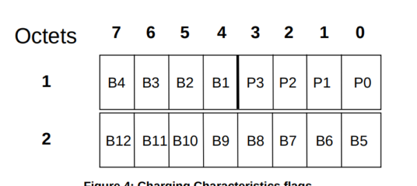
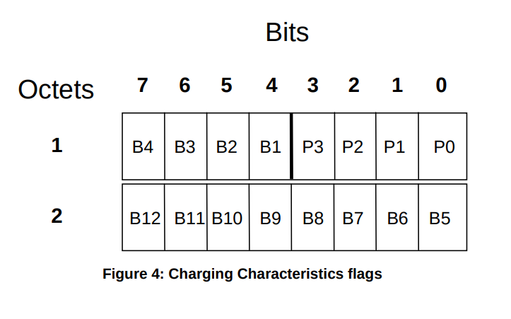
Charging Characteristics consists of a string of 16 bits designated as Profile (P) and Behaviour (B), shown in Figure 4. The first four bits (P) shall be used to select different charging trigger profiles, where each profile consists of the following trigger sets:
S-CDR: activate/deactivate CDRs, time limit, volume limit, maximum number of charging conditions, tariff times;
G-CDR: same as SGSN, plus maximum number of SGSN changes;
M-CDR: activate/deactivate CDRs, time limit, and maximum number of mobility changes;
SMS-MO-CDR: activate/deactivate CDRs;
SMS-MT-CDR: active/deactivate CDRs.
The Charging Characteristics field allows the operator to apply different kind of charging methods in the CDRs. A subscriber may have Charging Characteristics assigned to his subscription. These characteristics can be supplied by the HLR to the SGSN as part of the subscription information, and, upon activation of a PDP context, the SGSN forwards the charging characteristics to the GGSN on the Gn / Gp reference point according to the rules specified in Annex A of TS 32.251 [11].
This information can be used by the GSNs to activate CDR generation and control the closure of the CDR or the traffic volume containers (see clause 5.1.2.2.23) and is included in CDRs transmitted to nodes handling the CDRs via the Ga reference point. It can also be used in nodes handling the CDRs (e.g., the CGF or the billing system) to influence the CDR processing priority and routing.
These functions are accomplished by specifying the charging characteristics as sets of charging profiles and the expected behaviour associated with each profile.
The interpretations of the profiles and their associated behaviours can be different for each PLMN operator and are not subject to standardisation. In the present document only the charging characteristic formats and selection modes are specified.
The functional requirements for the Charging Characteristics as well as the profile and behaviour bits are further defined in normative Annex A of TS 32.251 [11], including the definitions of the trigger profiles associated with each CDR type.
The format of charging characteristics field is depicted in Figure 4. Px (x =0..3) refers to the Charging Characteristics Profile index. Bits classified with a “B” may be used by the operator for non-standardised behaviour (see Annex A of TS 32.251 [11]).
Right, well hopefully next time someone goes looking for this info you’ll find it a bit more easily than I did!
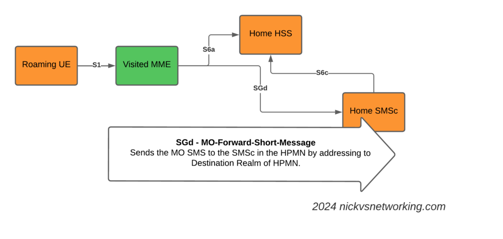
SGs-AP which is used for CSFB & SMS doesn’t span network borders (you can’t roam with SGs-AP), and with SMSoIP out of the question, that gave us the option of MAP or Diameter, so we picked Diameter.
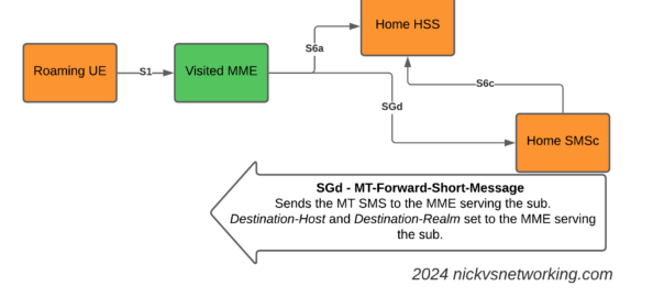
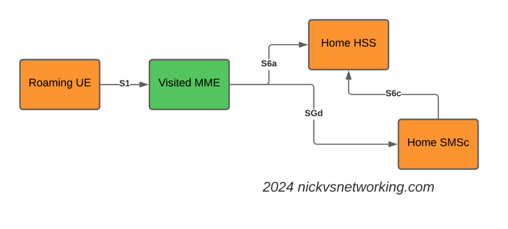
This introduces the S6c and SGd Diameter interfaces, in the diagrams below Orange is the Home Network (HPMN) and the Green is the Visited Network (VPMN).
The S6c interface is used between the SMSc and the HSS, in order to retrieve the routing information. This like the SRI-for-SM in MAP.
The SGd interface is used between the MME serving the UE and the SMSc, and is used for actual delivery of the MO/MT messages.
I haven’t shown the Diameter Routing Agents in these diagrams, but in reality there would be a DRA on the VPLMN and a DRA on the HPMN, and probably a DRA in the IPX between them too.
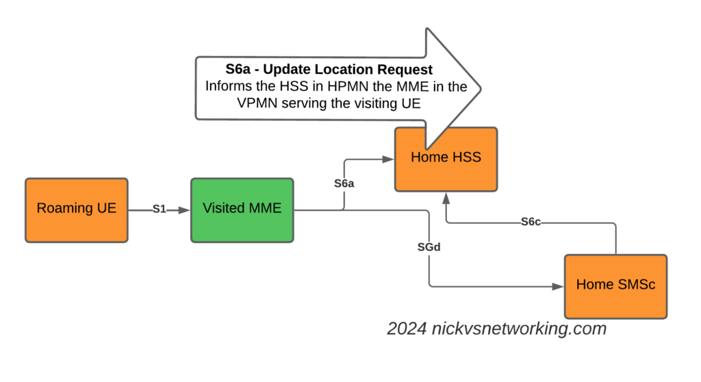
The Attach
The attach looks like a regular roaming attach, the MME in the Visited PMN sends an Update Location Request to the HSS, so the HSS knows the MME that is serving the subscriber.
S6a Update Location Request to indicate the MME serving the Subscriber
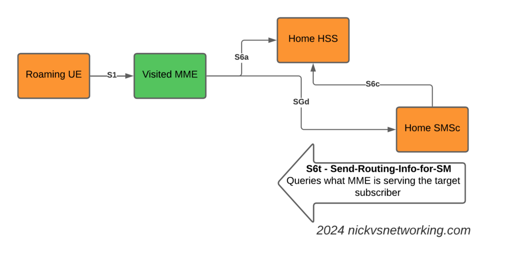
The Mobile Terminated SMS Flow
Now we introduce the S6c interface and the SGd interfaces.
When the Home SMSc has a message to send to the subscriber (Mobile Terminated SMS) it runs a the Send-Routing-Info-for-SM-Request (SRR) dialog to the HSS.
The Send-Routing-Info-for-SM-Answer (SRA) back from the HSS contains the info on the MME Diameter Host name and Diameter Realm serving the subscriber.
S6t – Send-Routing-Info-for-SM request to get the MME serving the subscriber
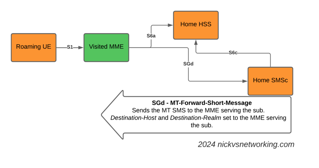
With this info, we can now craft a Diameter Request that will get sent to the MME serving the subscriber, containing the SMS PDU to send to the UE.
SGd MT-Forward-Short-Message to deliver Mobile Terminated SMS to the serving MME
We make sure it’s sent to the correct MME by setting the Destination-Host and Destination-Realm in the Diameter request.
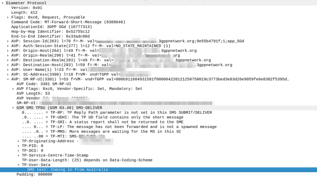
Here’s how the request looks from the SMSc towards our DRA:
As you can see the Destination Realm and Destination-Host is set, as is the User-Name set to the IMSI of the UE we want to send the message to.
And down the bottom you can see the SMS-TPDU, the same as it’s been all the way back since GSM days.
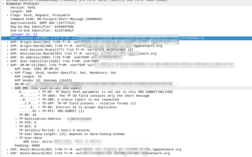
The Mobile Originated SMS Flow
The Mobile Originated flow is even simpler, because we don’t need to look up where to route it to.
The MME receives the MO SMS from the UE, and shoves it into a Diameter message with Application ID set to SGd and Destination-Realm set to the HPMN Realm.
When the message reaches the DRA in the HPMN it forwards the request to an SMSc and then the Home SMSc has the message ready to roll.
Android, being open source, allows us to see how this logic works, and it’s important for operators to understand this logic, as it’s what dictates the behavior in many scenarios.
It’s important to note that I’m not covering Apple here, this information is not publicly available to share for iOS devices, so I won’t be sharing anything on this – Apple has their own ecosystem to handle emergency calling, if you’re from an operator and reading this, I’d suggest getting in touch with your Apple account manager to discuss it, they’re always great to work with.
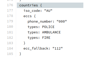
The Android Open Source Project has an “emergency number database”. This database has each of the emergency phone numbers and the corresponding service, for each country.
This file can be read at packages/services/Telephony/ecc/input/eccdata.txt on a phone with engineering mode.
Let’s take a look what’s in mainline Android for Australia:
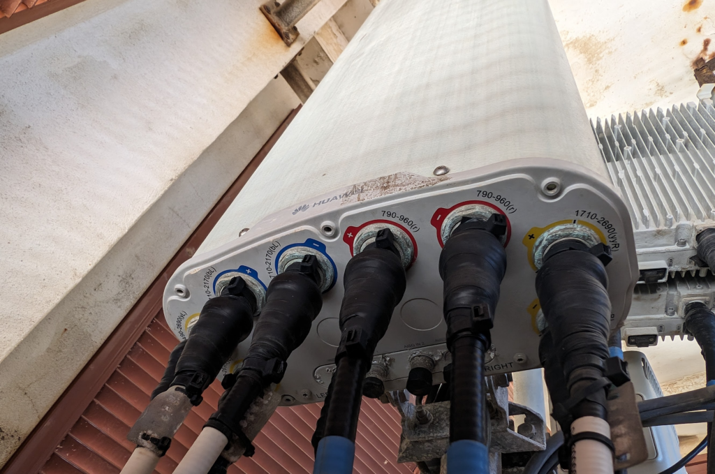
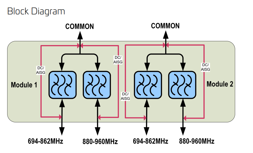
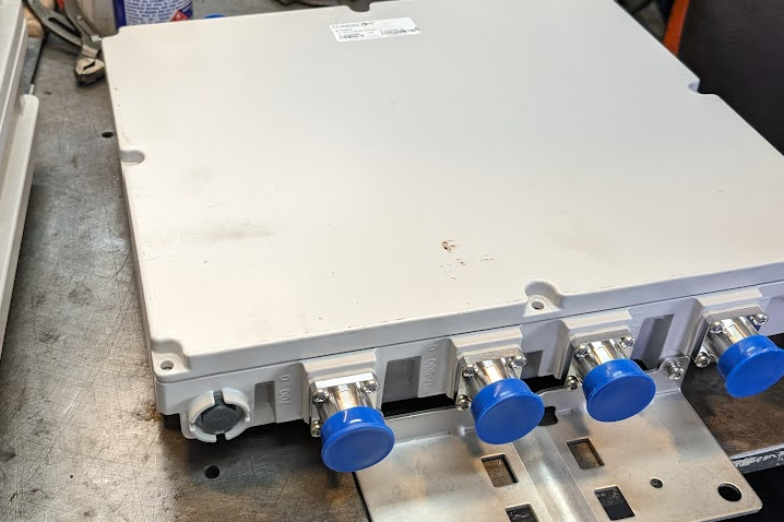
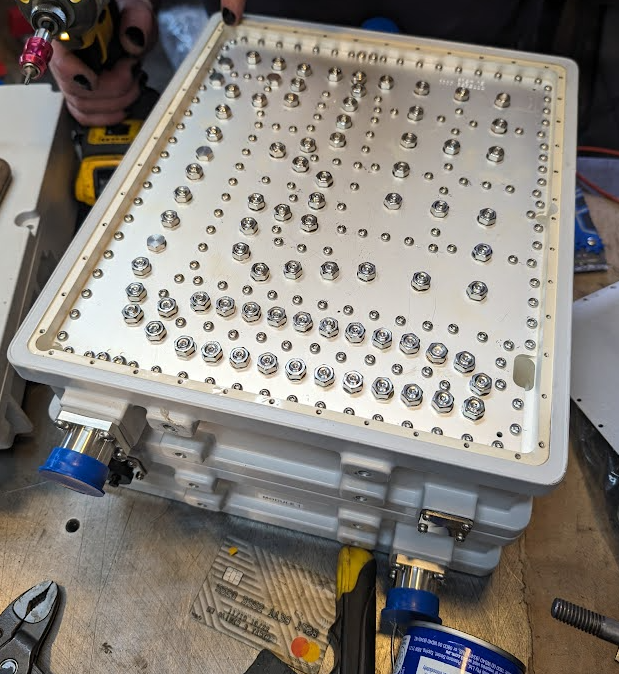
I recently ended up with a few Commscope RF combiners from a cell site, they’re not on frequencies that are of any use to us, so, let’s see what’s inside.
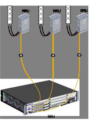
The units on the bench are Commscope Diplexer units, these ones allow you to put a signal between 694-862Mhz, and another signal between 880-960Mhz, on the same RF feeder up the tower.
It’s a nifty trick from the days where radio units lived at the bottom of the tower, but now with Remote Radio Units, and Active Antenna Units, it’s becoming increasingly uncommon to have radio units in the site hut, and more common to just run DC & fibre up the tower and power a radio unit right next to the antenna – This is especially important for higher frequencies where of course the feeder loss is greater.
Diplexer unit before it is maimed…
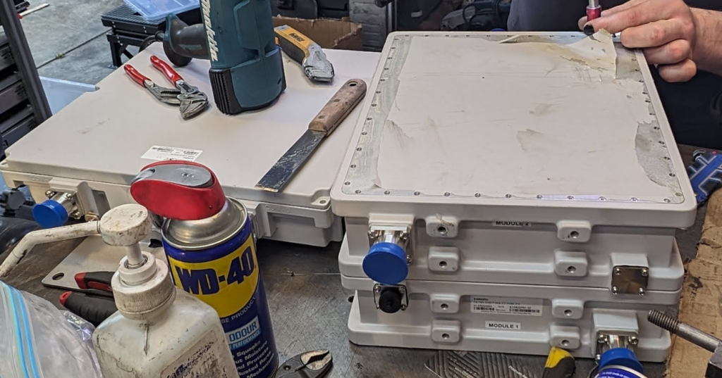
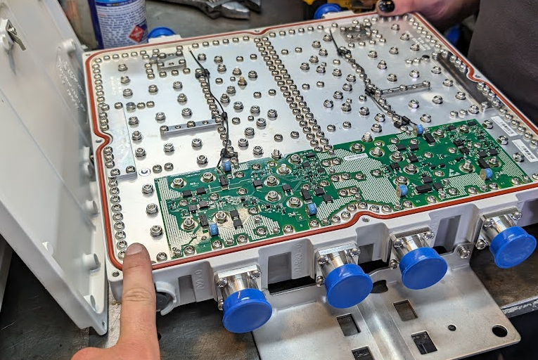
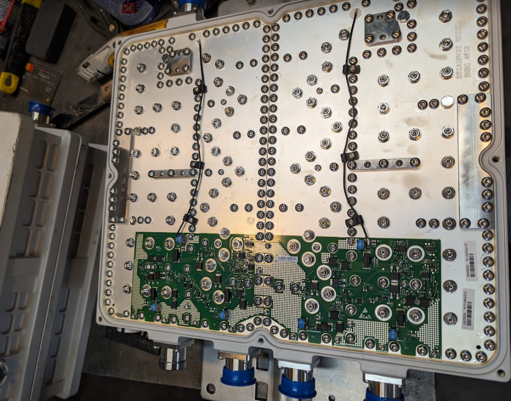
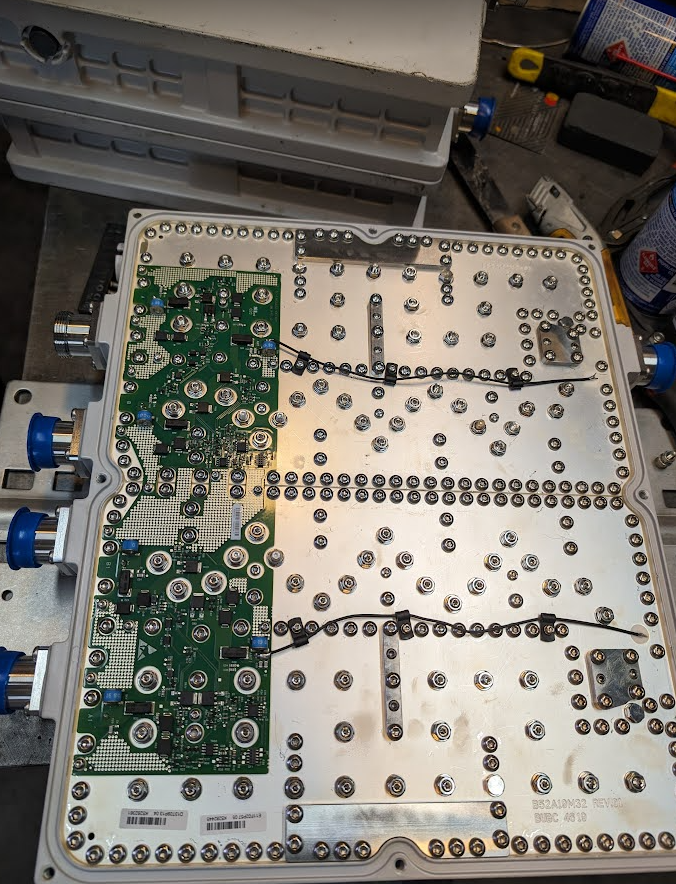
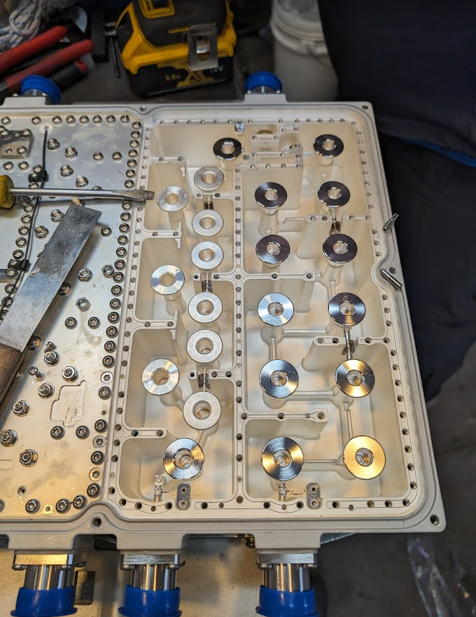
Anywho, that’s about all I know of them, after the liberal application of chemicals to remove the stickers and several burns from a heat gun, we started to get the unit open, to show the zillion adjustment bolts, and finely machined parts.
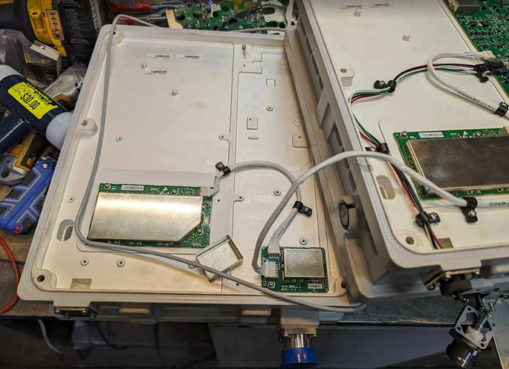
A lot of screwsBonus TMA
Thanks to Oliver for offering up the bench space when I rocked to up to their house with some stuff to pull apart.