In the past I had my iFCs setup to look for the P-Access-Network-Info header to know if the call was coming from the IMS, but it wasn’t foolproof – Fixed line IMS subs didn’t have this header.
If you work with FreeSWITCH there’s a good chance every time you do, you run fs_cli and attempt to read the firehose of data shown when making a call to make sense of what’s going on and why what you’re trying to do isn’t working.
That’s because we’ve edited the event_socket.conf.xml file, and fs_cli uses the event socket to connect to FreeSWITCH as well.
But there’s a simple fix,
Create a new file in /etc/fs_cli.conf and populate it with the info needed to connect to your ESL session you defined in event_socket.conf.xml, so if this is is your
[default]
; Put me in /etc/fs_cli.conf or ~/.fs_cli_conf
;overide any default options here
loglevel => 6
log-uuid => false


host     => 10.98.0.76
port     => 8021
password => mysupersecretpassword
debug    => 7
And that’s it, now you can run fs_cli and connect to the terminal once more!
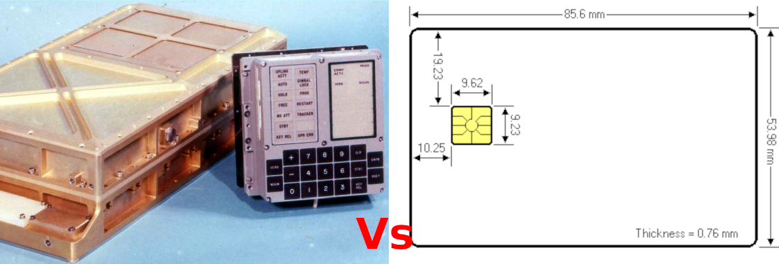
The first thing people learn about SIMs or the Smart Cards that the SIM / USIM app runs on, is that “There’s a little computer in the card”. So how little is this computer, and what’s the computing power in my draw full of SIMs?
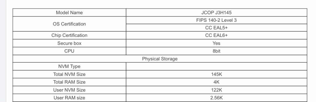
So for starters the SIM manufacturers love their NDAs, so I can’t post the chip specifications for the actual cards in my draw, but here’s some comparable specs from a seller selling Java based smart cards online:
Specs for Smart Card
4K of RAM is 4069 bytes. For comparison the Apollo Guidance Computer had 2048 words of RAM, but each “word” was 16 bits (two bytes), so actually this would translate to 4069 bytes so equal with one of these smart cards in terms of RAM – So the smart card above is on par with the AGC that took humans to the moon in terms of RAM, althhough the SIMs would be a wee bit larger if they were also using magnetic core memory like the AGC!
The Nintendo Entertainment System was powered by a MOS Technology 6502, it had access to 2K of RAM, two the Smart Card has twice as much RAM as the NES, so it could get you to the moon and play Super Mario Bros.
What about comparing Non-Volatile Memory (Storage)? Well, the smart card has 145KB of ROM / NVM, while Apollo flew with 36,864 words of RAM, each word is two bits to 73,728 Bytes, so roughly half of what the Smart Card has – Winner – Smart Card, again, without relying on core rope memory like AGC.
SIM cards are clocked kinda funkily so comparing processor speeds is tricky. Smart Cards are clocked off the device they connect to, which feeds them a clock signal via the CLK pin. The minimum clock speed is 1Mhz while the max is 5Mhz.
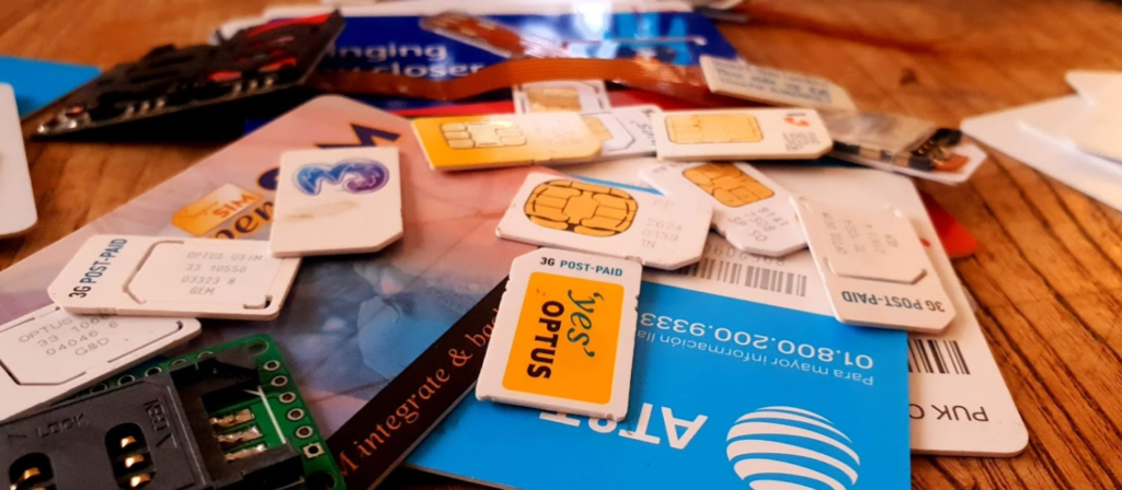
Now I’m somewhat of a hoarder when it comes to SIM Cards; in the course of my work I have to deal with a lot of SIMs…
Generally when we’re getting SIMs manufactured, during the Batch Approval Process (BAP) the SIM vendor will send ~25 cards for validation and testing. It’s not uncommon to go through several revisions. I probably do 10 of these a year for customers, so that’s 250 cards right there.
Then when the BAP is done I’ll get another 100 or so production cards for the lab, device testing, etc, this probably happens 3 times a year.
So that’s 550 SIMs a year, I do clean out every so often, but let’s call it 1000 cards in the lab in total.
In terms of ROM that gives me a combined 141.25 MB, I could store two Nintendo 64 games, or one Mini CD of data, stored across a thousand SIM cards – And you thought installing software from a few floppies was a pain in the backside, imagine accessing data from 1000 Smart Cards!
What about tying the smart cards together to use as a giant RAM BUS? Well our 1000 cards give us a combined 3.91 MB of RAM, well that’d almost be enough to run Windows 95, and enough to comfortably run Windows 3.1.
Practical do do any of this? Not at all, now if you’ll excuse me I think it’s time I throw out some SIMs…
It’s 1986 and you’ve got a 31 tons of copper, in the form of a giant 46 meter tall statue, that’s looking a bit worse for wear.
The Statue of Liberty has had water pooling in some areas, causing areas of her copper skin to corrode, and in some cases wearing all the way through.
On the other side of the iron curtain (it’s still up after all) there are probably quite a number of folks experienced in looking after giant statues, but alas, you’re the US National Parks Service and seeking help from the Soviets is probably a bad look.
The statue is made of Copper, and who knows more about copper than the phone company, with a vast, vast network of copper lines spanning the country?
So the National Parks Service called upon Bell Labs to help.
The Bell Labs’ chemists assigned to the project quickly pointed out that just replacing the corroded copper with new copper would hardly blend in – You’d have the shiny brown copper colour in the new sections, which wouldn’t match the verdigris that occurs through the oxidation of the copper, which would take years to form. (When she was delivered, the statue had a copper colour like you’d see in Copper piping, not the green patina we see today.)
Bell Labs staff looked at artificially creating the patina with acid solutions, to speed up the process to match the new copper with the old, but it was found it may cause structural weak points.
John Franey who was a technical assistant working at Bell Labs’ Murray Hill laboratories must have looked up at the roof of their buildings, constructed in 1941, and thought “Well that looks pretty close…”, so the naturally patinaed roof of Bell Lab’s New Jersey campus was peeled up and sent off for patching the statue.
Modern day roof at Murray Hill now with the verdigris that’s had 40 years to form
Murray Hill got a shiny new copper roof to replace the old green one they’d just given up, and the particles of copper corrosion scraped off the dismantled roof of a Bell Labs were mixed with acetone into a special spray used as concealer on the statue’s skin.
In exchange, Bell Labs staff were given some of the copper plates removed from the statue, so they could study the natural corrosion process in copper, in various weather conditions, which in turn would lead to a better understanding of how to build and maintain their copper plant.
If you’ve ever worked in roaming, you’ll probably have had the misfortune of dealing with Transferred Account Procedures aka TAP files.
It’s used for billing a 2G GSM call right up to 5G data usage, if you use a service while roaming, somewhere in the world there’s a TAP file with your usage in it.
A brief history of TAP
TAP was originally specified by the GSMA in 1991 as a standard CDR interchange format between operators, for use in roaming scenarios.
Notice I said GSMA – Not 3GPP – This means there’s no 3GPP TS docs for this, it’s defined by the industry lobby group’s members, rather than the standards body.
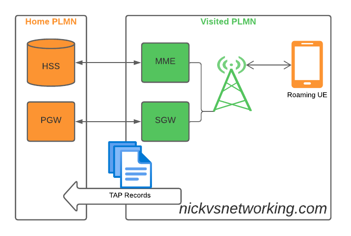
So what does this actually mean? Well, if you’re MNO A and a customer from MNO B roams into your network, all the calls, SMS and data consumed by the roaming subscriber from MNO B will need to be billed to MNO B, by you, MNO A.
If a network operator wants to get paid for traffic used on their network by roaming subscribers, they’d better send out a TAP file to the roamer’s home network.
TAP is the file format generated my MNO A and sent to MNO B, containing all the usage charges that subscribers from MNO B have racked up while roaming into your network.
These are broken down into “Transactions” (CDRs), for events like making a call, connecting a PDN session and consuming data, or sending a text.
In the beginning of time, GSM provided only voice calling service. This meant that the only services a subscriber could consume while roaming was just making/receiving voice calls which were billed at the end of each month. – This meant billing was equally simple, every so often the visisted network would send the TAP files for the voice calls made by subscribers visited other networks, to the home networks, which would markup those charges, and add them onto the monthly invoice for each subscriber who was roaming.
But of course today, calling accounts for a tiny amount of usage on the network, but this happened gradually while passing through the introduction of SMS, CAMEL services, prepaid services, mobile data, etc. For all these services that could be offered, the TAP format had to evolve to handle each of these scenarios.
As we move towards a flat IP architecture, where voice calls and SMS sent while roaming are just data, TAP files for 4G and 5G networks only need to show data transactions, so the call objects, CAMEL parameters and SMS objects are all falling by the wayside.
What’s inside a TAP File
TAP uses the most beloved of formats – ASN1 to encode the data. This means it is strictly formatted and rigidly specified.
Each file contains a Sequence Number which is a monotonically increasing number, which allows the receiver to know if any files have been missed between the file that’s being currently parsed, an the previous file.
They also have a recipient and sender TADIG code, which is a code allocated by GSMA that uniquely identifies the sender and the recipient of the file.
The TAP records exist in one of two common format, Notification Records and transferBatch records.
These files are exchanged between operators, in practice this means “Dumped on an FTP server as agreed between the two”.
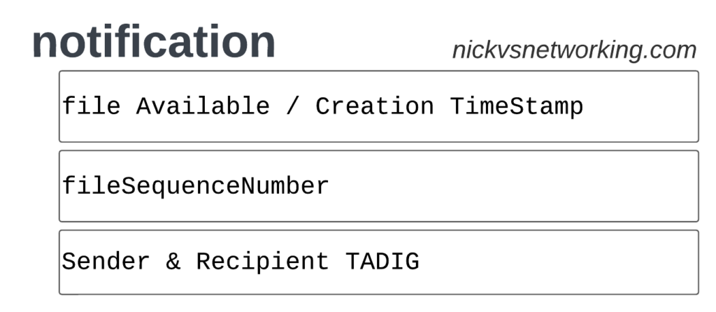
TAP Notification Records
Notifications are the simplest of TAP records and are used when there aren’t any CDRs for roaming events during the time period the TAP file covers.
These are essentially blank TAP files generated by the visited network to let the home network know it’s still there, but there are no roaming subs consuming services in that period.
Notification files are really simple, let’s take a look as one shown as JSON:
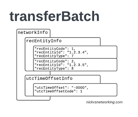
When we have services to bill and records to charge, that’s when instead we generate a transferBatch record.
It looks something like this:
There’s a lot going on in here, so let’s break it down section by section.
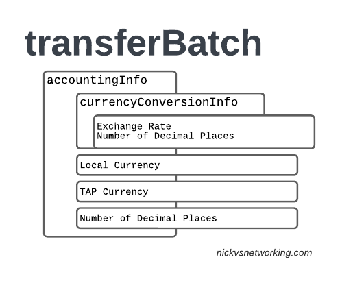
accountingInfo
The accountingInfo section specifies the currency, exchange rate parameters.
Keep in mind a TAP record generated by an operator in the US, would use USD, while the receiver of the file may be a European MNO dealing in EUR.
This gets even more complicated if you’re dealing with more obscure currencies where an intermediary currency is used, that’s where we bring in SDRs (“Special Drawing Right”) that map to the dollar value to be charged, kinda – the roaming agreement defines how many SDRs are in a dollar, in the example below we’re not using any, but you do see it.
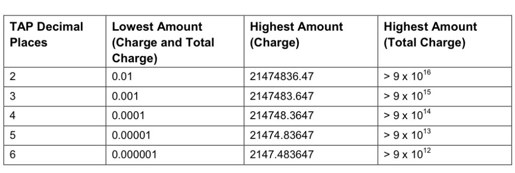
When it comes to numbers and decimal places, TAP doesn’t exactly make it easy.
Significant Digits are defined by counting the first number before the decimal point and all the numbers to the right of the decimal point, so for example the number 1.234 would be 4 significant digits (1 digit before the decimal point and 3 digits after it).
Decimal Places are not actually supported for the Value fields in the TAP file. This is tricky because especially today when roaming tariffs are quite low, these values can be quite small, and we need to represent them as an integer number. TAP defines decimal places as the number of digits after the decimal place.
When it comes to the maximum number of decimal places, this actually impacts the maximum number we can store in the field – as ASN1 strictly enforce what we put in it.
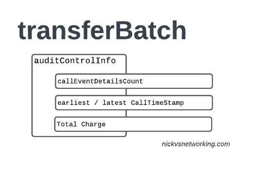
The auditControlInfo section contains the number of CDRs (callEventDetailsCount) contained in the TAP file, the timestamp of the first and last CDR in the file, the total charge and any tax charged.
All of the currency information was provided in the accountingInfo so this is just giving us our totals.
A CDR has 30 days from the time it was generated / service consumed by the roamer, to be baked into a TAP file. After this we can no longer charge for it, so it’s important that the earliestCallTimeStamp is not more than 30 days before the fileCreationTimeStamp seen in batchControlInfo.
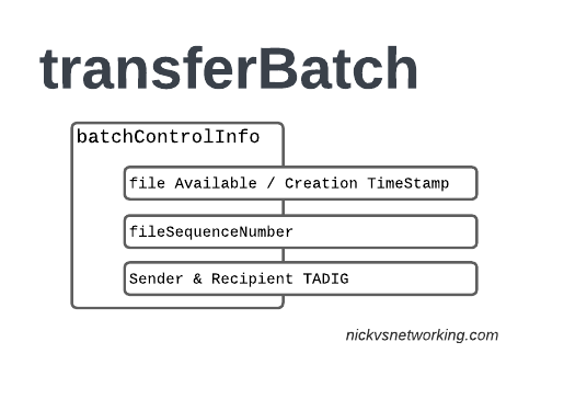
batchControlInfo
The batchControlInfo section specifies the time the TAP file became available for transfer, the time the file was created (usually the same), the sequence number and the sender / recipient TADIG codes.
As mentioned earlier, we track sequence number so the receiver can know if a TAP file has been missed; for example if you’ve got TAP file 1 and TAP file 3 comes in, you can determine you’ve missed TAP file 2.
Now we’re getting to the meat & potatoes of our TAP record, the CDRs themselves.
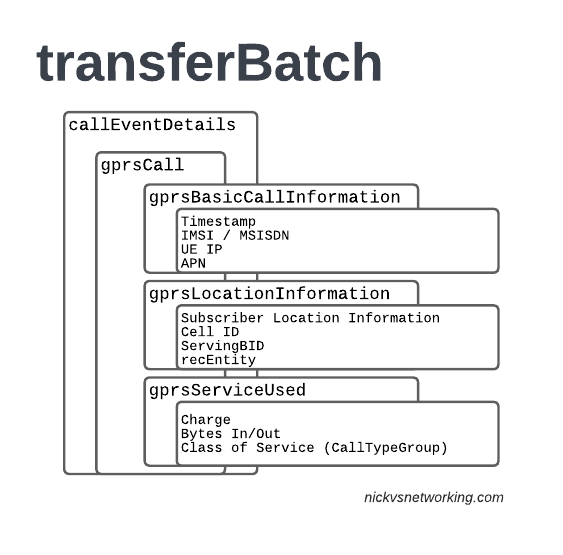
In LTE networks these are just records of data consumption, so let’s take a look inside the gprsCall records under callEventDetails:
In the gprsBasicCallInformation we’ve got as the name suggests the basic info about the data usage event. The time when the session started, the charging ID, the IMSI and the MSISDN of the subscriber to charge, along with their IP and the APN used.
Next up we have the gprsLocationInformation – rates and tariffs may be set based on the location of the subscriber, so we need to identify the area the sub was using the services to select correct tariff / rate for traffic in this destination.
The recEntity is the index number of the SGW / PGW used for the transaction (more on that later).
Next we have the gprsServiceUsed which, again as the name suggests, details the services used and the charge.
chargeDetailList contains the charged data (Made up of dataVolumeIncoming + dataVolumeOutgoing) and the cost.
The chargeableUnits indicates the actual data consumed, however most roaming agreements will standardise on some level of rounding, for example rounding up to the nearest Kilobyte (1024 bytes), so while a sub may consume 1025 bytes of data, they’d be billed for 2045 bytes of data. The data consumed is indicated in the chargeableUnits which indicates how much data was actually consumed, before any rounding policies where applied, while the amount that is actually charged (When taking into account rounding policies) isindicated inside Charged Units.
In the example below data usage is rounded up to the nearest 1024 bytes, 134390 bytes rounds up to the nearest 1024 gives you 135168 bytes.
As this is data we’re talking bytes, but not all bytes are created equal!
VoLTE traffic, using a QCI1 bearer is more valuable than QCI 9 cat videos, and TAP records take this into account in the Call Type Groups, each of which has a different price – Call Type Level 1 indicates the type of traffic, for S8 Home Routed LTE Traffic this is 10 (HGGSN/HP-GW), while Call Type Level 2 indicates the type of traffic as mapped to QCI values:
So Call Type Level 2 set to 20 indicates that this is “20 Unspecified/default LTE QCIs”, and Call Type Level 3 can be set to any value based on a defined inter-operator tariff.
recEntityType 7 means a PGW and contains the IP of the PGW in the Home PLMN, while recEntityType 8 means SGW and is the SGW in the Visited PLMN.
So this means if we reference recEntityCode 2 in a gprsCall, that we’re referring to an SGW at 1.2.3.5.
Lastly also got the utcTimeOffsetInfo to indicate the timezones used and assign a unique code to it.
Using the Records
We as humans? These records aren’t meant for us.
They’re designed to be generated by the Visited PLMN and sent to to the home PLMN, which ingests it and pays the amount specified in the time agreed.
Generally this is an FTP server that the TAP records get dumped into, and an automated bank transfer job based on the totals for the TAP records.
Testing of the TAP records is called “TADIG Testing” and it’s something we’ll go into another day, but in essence it’s validating that the output and contents of the files meet what both operators think is the contract pricing and specifications.
So that’s it! That’s what’s in a TAP record, what it does and how we use it!
GSMA are introducing BCE – Billing & Charging Evolution, a new standard, designed to last for the next 30+ years like TAP has. It’s still in its early days, but that’s the direction the GSMA has indicated it would like to go.
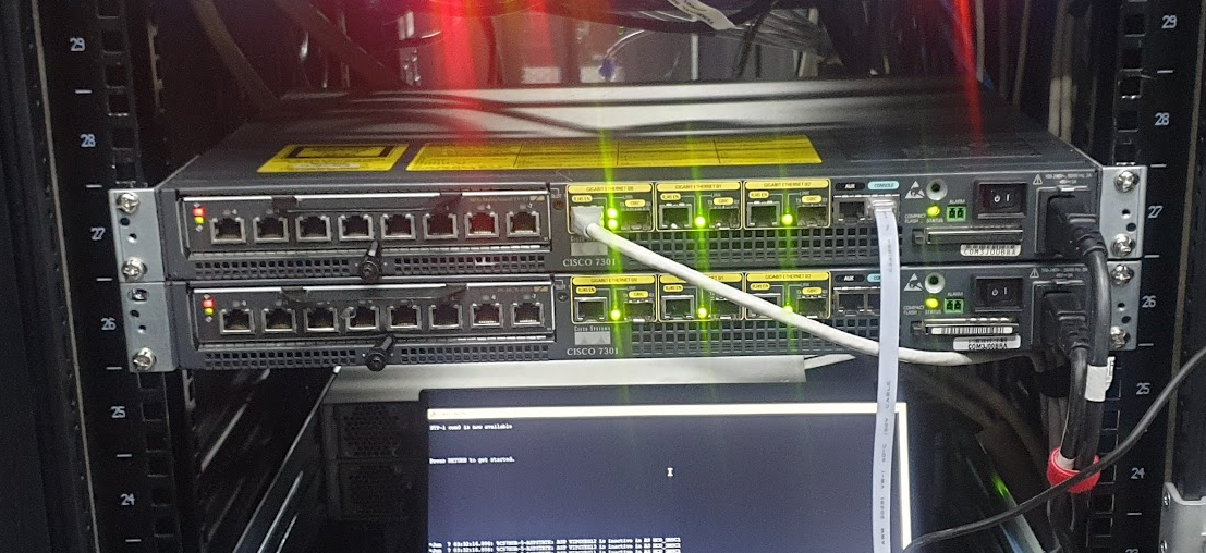
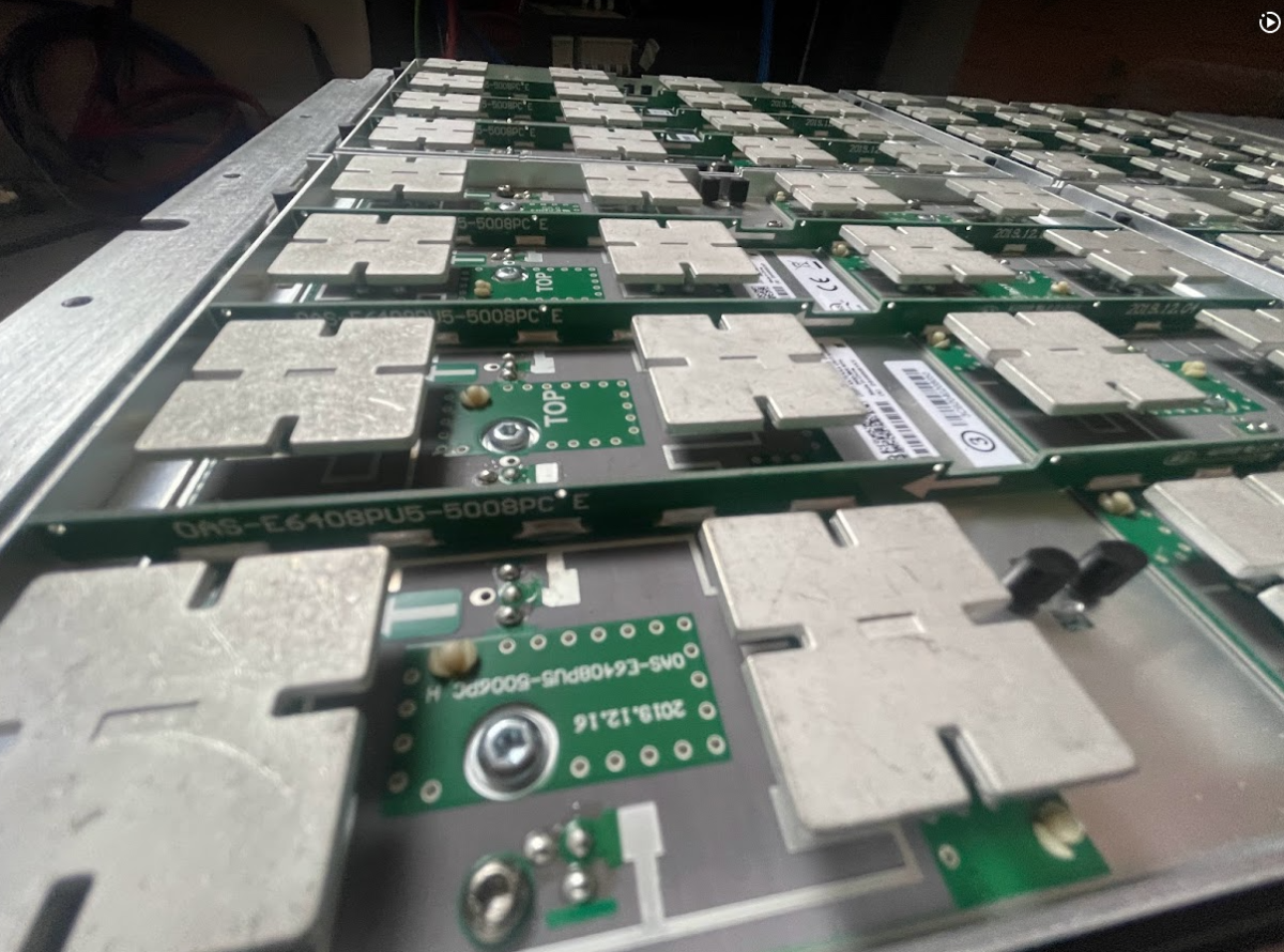
For the past few months I’ve had a Band 78 NR active antenna unit sitting next to my desk.
It’s a very cool bit of kit that doesn’t get enough love, but I thought I’d pop open the radome and take a peek inside.
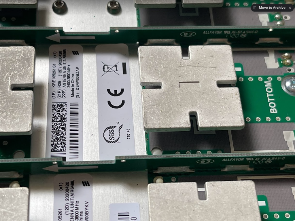
Individual antenna elements
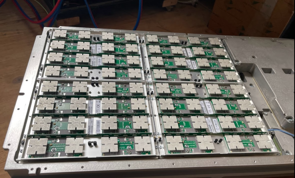
What I found very interesting is that it’s not all antennas in there!
… 29, 30, 31, 32. Yup. Checks out.
There are the expected number of antennas (I mean if I opened it up and found 31 antennas I’d have been surprised) but they don’t take up the whole volume of the unit, only about half,
AAU with Radome reinstalled
Well, after that strip show, back to sitting in my office until I need to test something 5G SA again…
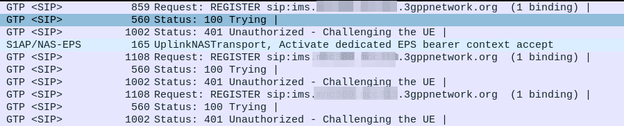
Everything was working on the IMS, then I go to bed, the next morning I fire up the test device and it just won’t authenticate to the IMS – The S-CSCF generated a 401 in response to the REGISTER, but the next REGISTER wouldn’t pass.
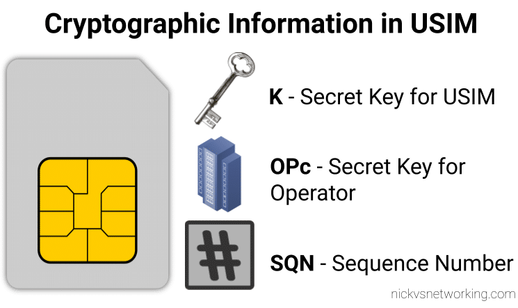
When we generate the vectors (for IMS auth and standard auth) one of the inputs to generate the vectors is the Sequence Number or SQN.
This SQN ticks over like an odometer for the number of times the SIM / HSS authentication process has been performed.
There is some leeway in the SQN – It may not always match between the SIM and the HSS and that’s to be expected. When the MME sends an Authentication-Information-Request it can ask for multiple vectors so it’s got some in reserve for the next time the subscriber attaches, and that’s allowed.
But there are limits to how far out our SQN can be, and for good reason – One of the key purposes for the SQN is to protect against replay attacks, where the same vector is replayed to the UE. So the SQN on the HSS can be ahead of the SIM (within reason), but it can’t be behind – Odometers don’t go backwards.
So the issue was with the SQN on the SIM being out of Sync with the SQN in the IMS, how do we know this is the case, and how do we fix this?
Well there is a resync mechanism so the SIM can securely tell the HSS what the current SQN it is using, so the HSS can update it’s SQN.
When verifying the AUTN, the client may detect that the sequence numbers between the client and the server have fallen out of sync. In this case, the client produces a synchronization parameter AUTS, using the shared secret K and the client sequence number SQN. The AUTS parameter is delivered to the network in the authentication response, and the authentication can be tried again based on authentication vectors generated with the synchronized sequence number.
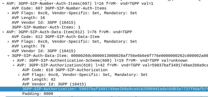
In our example we can tell the sub is out of sync as in our Multimedia Authentication Request we see the SIP-Authorization AVP, which contains the AUTS (client synchronization parameter) which the SIM generated and the UE sent back to the S-CSCF. Our HSS can use the AUTS value to determine the correct SQN.
SIP-Authorization AVP in the Multimedia Authentication Request means the SQN is out of Sync and this AVP contains the RAND and AUTN required to Resync
Note: The SIP-Authorization AVP actually contains both the RAND and the AUTN concatenated together, so in the above example the first 32 bytes are the AUTN value, and the last 32 bytes are the RAND value.
So the HSS gets the AUTS and from it is able to calculate the correct SQN to use.
Then the HSS just generates a new Multimedia Authentication Answer with a new vector using the correct SQN, sends it back to the IMS and presto, the UE can respond to the challenge normally.
We’re doing more and more network automation, and something that came up as valuable to us would be to have all the IPs in HOMER SIP Capture come up as the hostnames of the VM running the service.
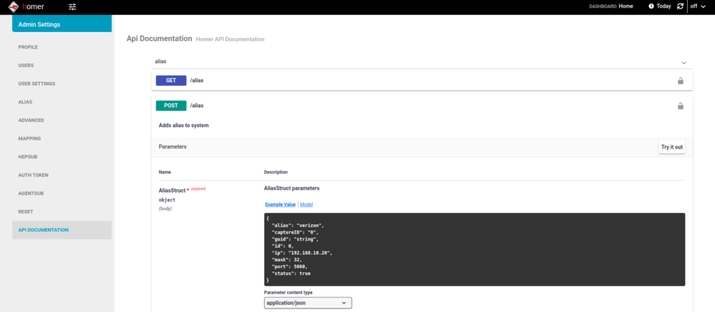
Luckily for us HOMER has an API for this ready to roll, and best of all, it’s Swagger based and easily documented (awesome!).
(Probably through my own failure to properly RTFM) I was struggling to work out the correct (current) way to Authenticate against the API service using a username and password.
Because the HOMER team are awesome however, the web UI for HOMER, is just an API client.
This means to look at how to log into the API, I just needed to fire up Wireshark, log into the Web UI via my browser and then flick through the packets for a real world example of how to do this.
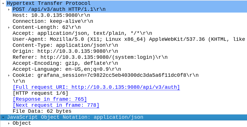
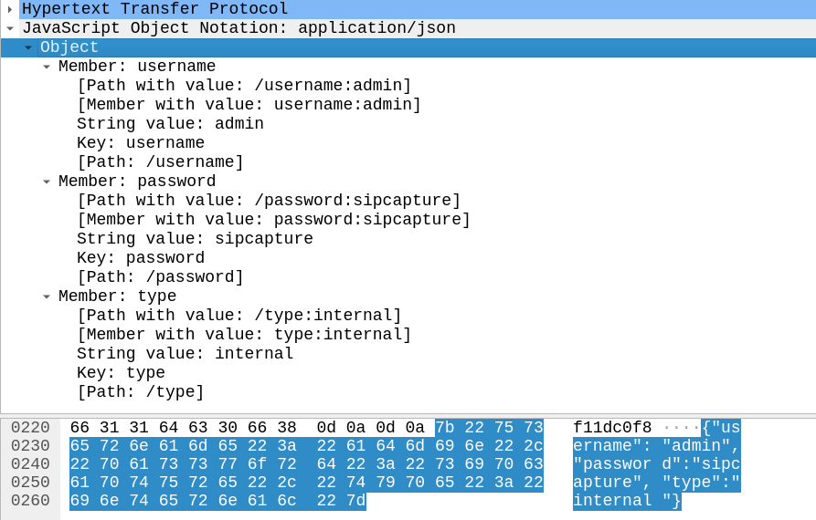
Homer Login JSON body as seen by Wireshark
In the Login action I could see the browser posts a JSON body with the username and password to /api/v3/auth
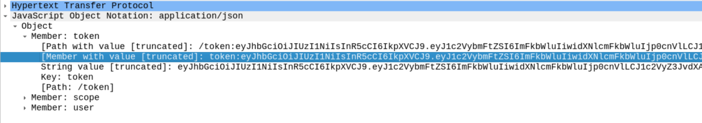
And in return the Homer API Server responds with a 201 Created an a auth token back:
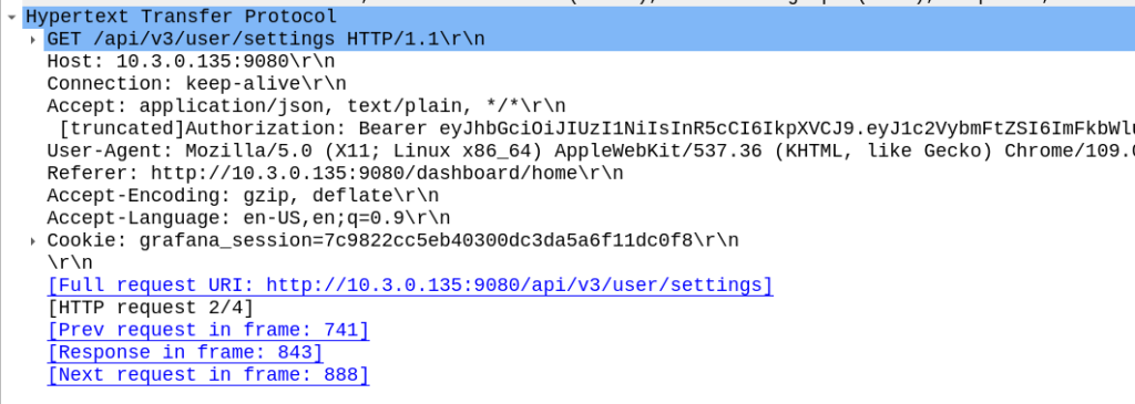
Now in order to use the API we just need to include that token in our Authorization: header then we can hit all the API endpoints we want!
For me, the goal we were setting out to achieve was to setup the aliases from our automatically populated list of hosts. So using the info above I setup a simple Python script with Requests to achieve this:
import requests
s = requests.Session()

#Login and get Token
url = 'http://homer:9080/api/v3/auth'
json_data = {"username":"admin","password":"sipcapture"}
x = s.post(url, json = json_data)
print(x.content)
token = x.json()['token']
print("Token is: " + str(token))


#Add new Alias
alias_json = {
          "alias": "Blog Example",
          "captureID": "0",
          "id": 0,
          "ip": "1.2.3.4",
          "mask": 32,
          "port": 5060,
          "status": True
        }

x = s.post('http://homer:9080/api/v3/alias', json = alias_json, headers={'Authorization': 'Bearer ' + token})
print(x.status_code)
print(x.content)


#Print all Aliases
x = s.get('http://homer:9080/api/v3/alias', headers={'Authorization': 'Bearer ' + token})
print(x.json())
And bingo we’re done, a new alias defined.
We wrapped this up in a for loop for each of the hosts / subnets we use and hooked it into our build system and away we go!
With the Homer API the world is your oyster in terms of functionality, all the features of the Web UI are exposed on the API as the Web UI just uses the API (something I wish was more common!).
Using the Swagger based API docs you can see examples of how to achieve everything you need to, and if you ever get stuck, just fire up Wireshark and do it in the Homer WebUI for an example of how the bodies should look.
Misunderstood, under appreciated and more capable than people give it credit for, is our PCRF.
But what does it do?
Most folks describe the PCRF in hand wavy-terms – “it does policy and charging” is the answer you’ll get, but that doesn’t really tell you anything.
So let’s answer it in a way that hopefully makes some practical sense, starting with the acronym “PCRF” itself, it stands for Policy and Charging Rules Function, which is kind of two functions, one for policy and one for rules, so let’s take a look at both.
Policy
In cellular world, as in law, policy is the rules.
For us some examples of policy could be a “fair use policy” to limit customer usage to acceptable levels, but it can also be promotional packages, services like “free Spotify” packages, “Voice call priority” or “unmetered access to Nick’s Blog and maximum priority” packages, can be offered to customers.
All of these are examples of policy, and to make them work we need to target which subscribers and traffic we want to apply the policy to, and then apply the policy.
Charging Rules
Charging Rules are where the policy actually gets applied and the magic happens.
It’s where we take our policy and turn it into actionable stuff for the cellular world.
Let’s take an example of “unmetered access to Nick’s Blog and maximum priority” as something we want to offer in all our cellular plans, to provide access that doesn’t come out of your regular usage, as well as provide QCI 5 (Highest non dedicated QoS) to this traffic.
To achieve this we need to do 3 things:
Profile the traffic going to this website (so we capture this traffic and not regular other internet traffic)
Charge it differently – So it’s not coming from the subscriber’s regular balance
Up the QoS (QCI) on this traffic to ensure it’s high priority compared to the other traffic on the network
So how do we do that?
Profiling Traffic
So the first step we need to take in providing free access to this website is to filter out traffic to this website, from the traffic not going to this website.
Let’s imagine that this website is hosted on a single machine with the IP 1.2.3.4, and it serves traffic on TCP port 443. This is where IPFilterRules (aka TFTs or “Traffic Flow Templates”) and the Flow-Description AVP come into play. We’ve covered this in the past here, but let’s recap:
IPFilterRules are defined in the Diameter Base Protocol (IETF RFC 6733), where we can learn the basics of encoding them,
They take the format:
action dir proto from src to dst
The action is fairly simple, for all our Dedicated Bearer needs, and the Flow-Description AVP, the action is going to be permit. We’re not blocking here.
The direction (dir) in our case is either in or out, from the perspective of the UE.
Next up is the protocol number (proto), as defined by IANA, but chances are you’ll be using 17 (UDP) or 6 (TCP).
The from value is followed by an IP address with an optional subnet mask in CIDR format, for example from 10.45.0.0/16would match everything in the 10.45.0.0/16 network.
Following from you can also specify the port you want the rule to apply to, or, a range of ports.
Like the from, the tois encoded in the same way, with either a single IP, or a subnet, and optional ports specified.
And that’s it!
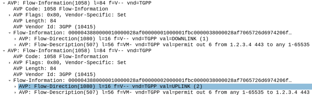
So let’s create a rule that matches all traffic to our website hosted on 1.2.3.4 TCP port 443,
permit out 6 from 1.2.3.4 443 to any 1-65535
permit out 6 from any 1-65535 to 1.2.3.4 443
All this info gets put into the Flow-Information AVPs:
With the above, any traffic going to/from 1.23.4 on port 443, will match this rule (unless there’s another rule with a higher precedence value).
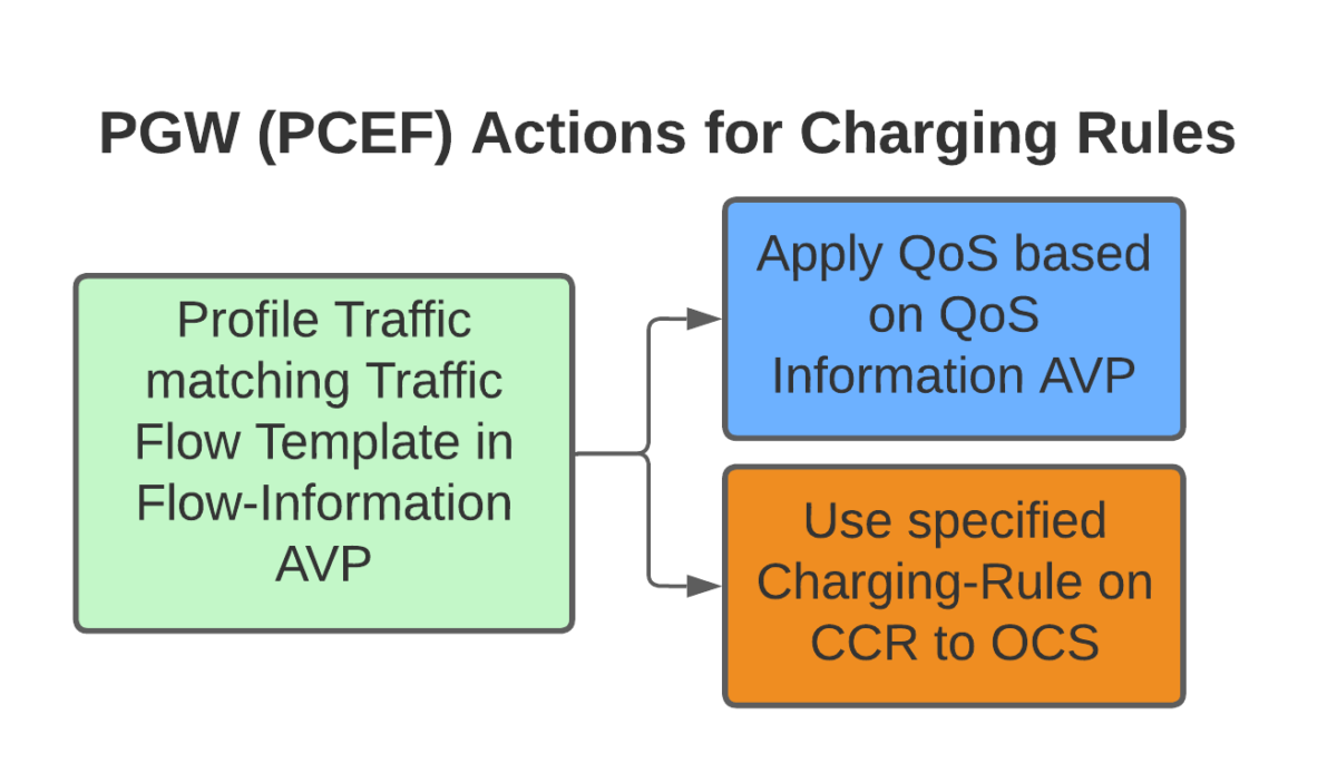
Charging Actions
So with our traffic profiled, the next question is what actions are we going to take, well there’s two, we’re going to provide unmetered access to the profiled traffic, and we’re going to use QCI 4 for the traffic (because you’ll need a guaranteed bit rate bearer to access!).
Charging-Group for Profiled Traffic
To allow for Zero Rating for traffic matching this rule, we’ll need to use a different Rating Group.
Let’s imagine our default rating group for data is 10000, then any normal traffic going to the OCS will use rating group 10000, and the OCS will apply the specific rates and policies based on that.
Rating Groups are defined in the OCS, and dictate what rates get applied to what Rating Groups.
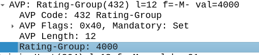
For us, our default rating group will be charged at the normal rates, but we can define a rating group value of 4000, and set the OCS to provide unlimited traffic to any Credit-Control-Requests that come in with Rating Group 4000.
This is how operators provide services like “Unlimited Facebook” for example, a Charging Rule matches the traffic to Facebook based on TFTs, and then the Rating Group is set differently to the default rating group, and the OCS just allows all traffic on that rating group, regardless of how much is consumed.
Inside our Charging-Rule-Definition, we populate the Rating-Group AVP to define what Rating Group we’re going to use.
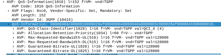
Setting QoS for Profiled Traffic
The QoS Description AVP defines which QoS parameters (QCI / ARP / Guaranteed & Maximum Bandwidth) should be applied to the traffic that matches the rules we just defined.
As mentioned at the start, we’ll use QCI 4 for this traffic, and allocate MBR/GBR values for this traffic.
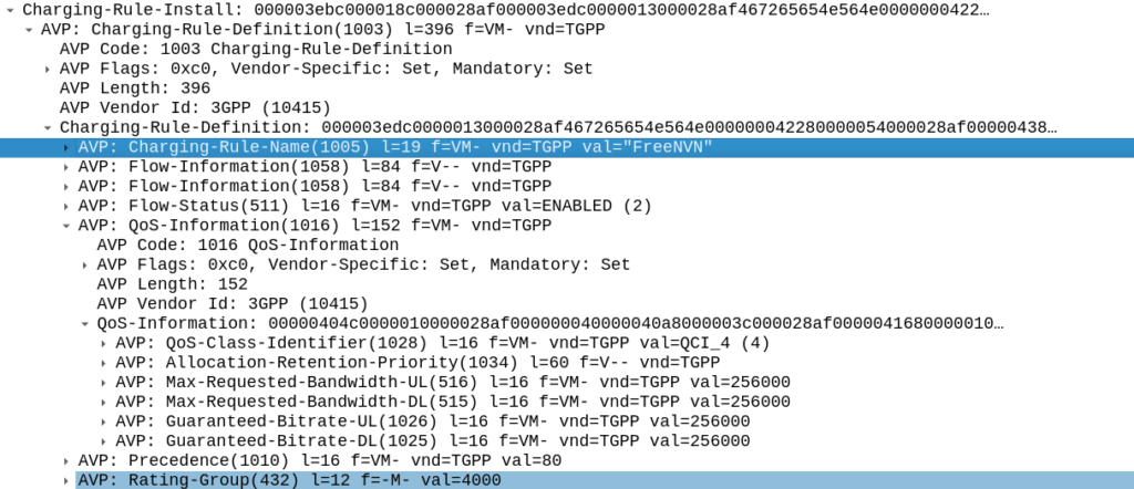
Putting it Together – The Charging Rule
So with our TFTs defined to match the traffic, our Rating Group to charge the traffic and our QoS to apply to the traffic, we’re ready to put the whole thing together.
So here it is, our “Free NVN” rule:
I’ve attached a PCAP of the flow to this post.
In our next post we’ll talk about how the PGW handles the installation of this rule.
One day recently I was messing with the XCAP server, trying to set the Call Forward timeout. In the process I triggered the UE to send a USSD request to the IMS.
Huh, I thought, “I wonder how hard it would be to build a USSD Gateway for our IMS?”, and this my friends, is the story of how I wasted a good chunk of my weekend trying (and failing) to add support for USSD.
You might be asking “Who still uses USSD?” – The use cases for USSD are pretty thin on the ground in this day and age, but I guess balance query, and uh…
But this is the story of what I tried before giving up and going outside…
Routing
First I’d need to get the USSD traffic towards the USSD Gateway, this means modifying iFCs. Skimming over the spec I can see the Recv-Info: header for USSD traffic should be set to “g.3gpp.ussd” so I knocked up an iFC to match that, and route the traffic to my dev USSD Gateway, and added it to the subscriber profile in PyHSS:
Easy peasy, now we have the USSD requests hitting our USSD Gateway.
The Response
I’ll admit that I didn’t jump straight to the TS doc from the start.
The first place I headed was Google to see if I could find any PCAPs of USSD over IMS/SIP.
And I did – Restcomm seems to have had a USSD product a few years back, and trawling around their stuff provided some reference PCAPs of USSD over SIP.
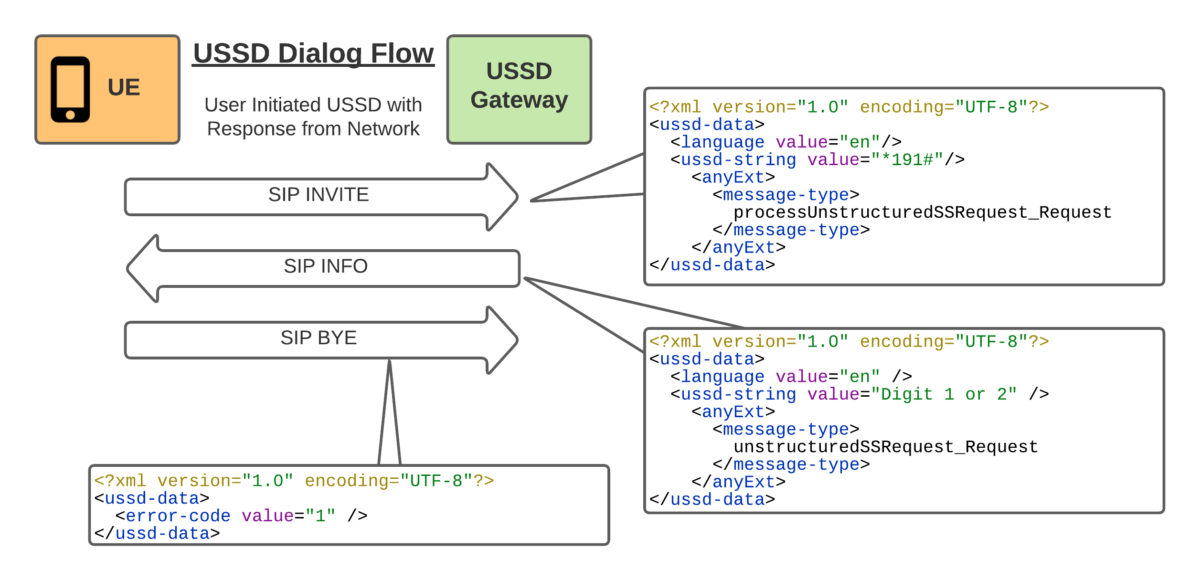
So the flow seemed pretty simple, SIP INVITE to set up the session, SIP INFO for in-dialog responses and a BYE at the end.
With all the USSD guts transferred as XML bodies, in a way that’s pretty easy to understand.
Being a Kamailio fan, that’s the first place I started, but quickly realised that SIP proxies, aren’t great at acting as the UAS.
So I needed to generate in-dialog SIP INFO messages, so I turned to the UAC module to generate the SIP INFO response.
My Kamailio code is super simple, but let’s have a look:
request_route {

        xlog("Request $rm from $fU");

        if(is_method("INVITE")){
                xlog("USSD from $fU to $rU (Emergency number) CSeq is $cs ");
                sl_reply("200", "OK Trying USSD Phase 1");      #Generate 200 OK
                route("USSD_Response"); #Call USSD_Response route block
                exit;
        }
}

route["USSD_Response"]{
        xlog("USSD_Response Route");
        #Generate a new UAC Request
        $uac_req(method)="INFO";
        $uac_req(ruri)=$fu;     #Copy From URI to Request URI
        $uac_req(furi)=$tu;     #Copy To URI to From URI
        $uac_req(turi)=$fu;     #Copy From URI to To URI
        $uac_req(callid)=$ci;   #Copy Call-ID
                                #Set Content Type to 3GPP USSD
        $uac_req(hdrs)=$uac_req(hdrs) + "Content-Type: application/vnd.3gpp.ussd+xml\r\n";
                                #Set the USSD XML Response body
        $uac_req(body)="<?xml version='1.0' encoding='UTF-8'?>
        <ussd-data>
                <language value=\"en\"/>
                <ussd-string value=\"Bienvenido. Seleccione una opcion: 1 o 2.\"/>
        </ussd-data>";
        $uac_req(evroute)=1;    #Set the event route to use on return replies
        uac_req_send();         #Send it!
}
So the UAC module generates the 200 OK and sends it back.
“That was quick” I told myself, patting myself on the back before trying it out for the first time.
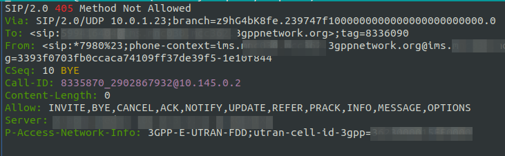
Huston, we have a problem – Although the Call-ID is the same, it’s not an in-dialog response as the tags aren’t present, this means our UE send back a 405 to the SIP INFO.
Right. Perhaps this is the time to read the Spec…
Okay, so the SIP INFO needs to be in dialog. Can we do that with the UAC module? Perhaps not…
But alas real life came back to rear its ugly head, and this adventure will have to continue another day…
Update: Thanks to a kindly provided PCAP I now know what I was doing wrong, and so we’ll soon have a follow up to this post named “Successes in cobbling together a USSD Gateway” just as soon as I have a weekend free.
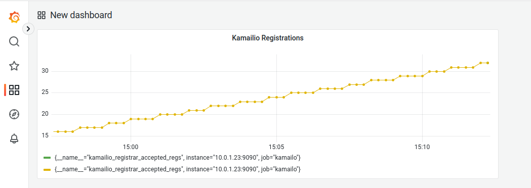
I recently fell in love with the Prometheus + Grafana combo, and I’m including it in as much of my workflow as possible, so today we’ll be integrating this with another favorite – Kamailio.
Why would we want to integrate Kamailio into Prometheus + Grafana? Observability, monitoring, alerting, cool dashboards to make it look like you’re doing complicated stuff, this duo have it all!
I’m going to assume some level of familiarity with Prometheus here, and at least a basic level of understanding of Kamailio (if you’ve never worked with Kamailio before, check out my Kamailio 101 Series, then jump back here).
So what will we achieve today?
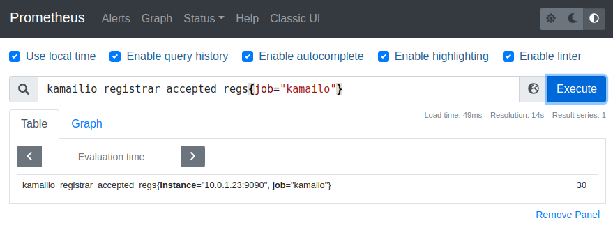
We’ll start with the simple SIP Registrar in Kamailio from this post, and we’ll add on the xhttp_prom module, and use it to expose some stats on the rate of requests, and responses sent to those requests.
So to get started we’ll need to load some extra modules, xhttp_prom module requires xhttp (If you’d like to learn the basics of xhttp there’s also a Kamailio Bytes – xHTTP Module post covering the basics) so we’ll load both.
xHTTP also has some extra requirements to load, so in the top of our config we’ll explicitly specify what ports we want to bind to, and set two parameters that control how Kamailio handles HTTP requests (otherwise you’ll not get responses for HTTP GET requests).
Then where you load all your modules we’ll load xhttp and xhttp_prom, and set the basic parameters:
loadmodule "xhttp.so"
loadmodule "xhttp_prom.so"

# Define two counters and a gauge
modparam("xhttp_prom", "xhttp_prom_stats", "all")
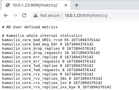
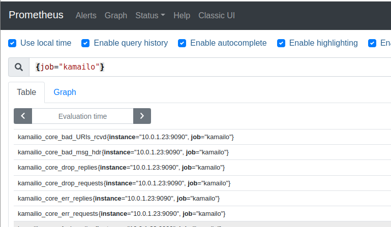
By setting xhttp_prom module to expose all stats, this exposes all of Kamailio’s internal stats as counters to Prometheus – This means we don’t need to define all our own counters / histograms / gauges, instead we can use the built in ones from Kamailio. Of course we can define our own custom ones, but we’ll do that in our next post.
Lastly we’ll need to add an event route to handle HTTP requests to the /metrics URL:
Yes, this is a lazy post. As the year draws to a close I was asked to put together a list of the most popular posts of the year.
Of the posts written this, year, there’s been a lot for people who build and work on networks to make their lives easier and their workflows more efficient.
The most popular posts this year weren’t actually from this year, this time last year I posted the Evolved Packet Core Analysis Challenge – The Skill-tester / Claw Machine of the Telecom world, test your EPC knowhow and skills!
As more and more readers are starting to work with 5GC this past year, My first 5G Core: Open5Gs and UERANSIM has been very popular as folks dip a toe in the water with 5GC.
On a personal notes, it looks like I finished every book in my reading list (Except Girdle Round the Earth that’s still on my bedside table), I did take a break from writing around the middle of the year, but weekly ish posts are coming back.
If you have a problem, if no one else can help, and if you can find me, drop me a line – [email protected] / LinkedIn / Twitter.
So far in our lab we’ve got connectivity between to points, but we’re not carrying any useful data on top of it.
In the same way that TCP is great, but what makes it really useful is carrying application layers like HTTP on top, MTP3 exists to facilitate carrying higher-layer protocols, like ISUP, MAP, SCCP, etc, so let’s get some traffic onto our network.
ISUP is the ISDN User Part, ISUP is used to setup and teardown calls between two exchanges / SSPs – it’s the oldest and the most simple SS7 application to show off, so that’s what we’ll be working with today.
If you’ve not dealt much with ISDN in the past, then that’s OK – we’re not going to deep dive into all the nitty gritty of how ISDN Signaling works, but we’ll just skim the surface to showing how SS7/Sigtran transports the ISUPpackets. So you can see how SS7 is used to transport this protocol.
You can think of it a lot like SIP, which is if not the child of ISUP, then it at least bares a striking resemblance.
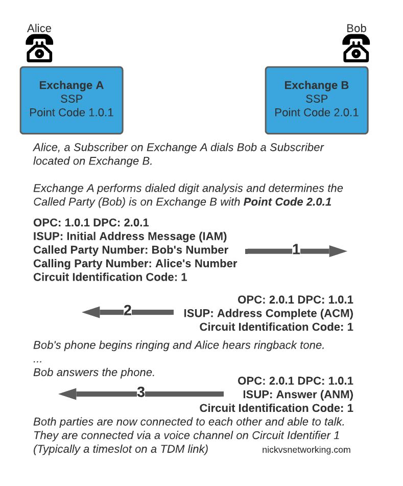
So let’s look at an ISUP call flow:
The call is initiated with an Initial Address Message (IAM), akin to a SIP INVITE, sent by the SSP/Exchange of the calling party to the SSP/Exchange of the called party. When the remote party starts to ring, the remote exchange sends an Address Complete (ACM), which is similar to a 100 TRYING in SIP. Once the remote party answers, the remote exchange sends back an Answer Message (ANM), and our call starts, just like a 200 OK.
Rather than SDP for transferring media, timeslots or predefined channels / circuits are defined, each identified by a number, which both sides will use for the media path.
Finally whichever side terminates the call will send a Release (REL) message, which is confirmed with the Release Complete (RLC).
I told you we’d be quick!
So that’s the basics of ISUP, in our next post we’ll do some PCAP analysis on real world ISUP flows!
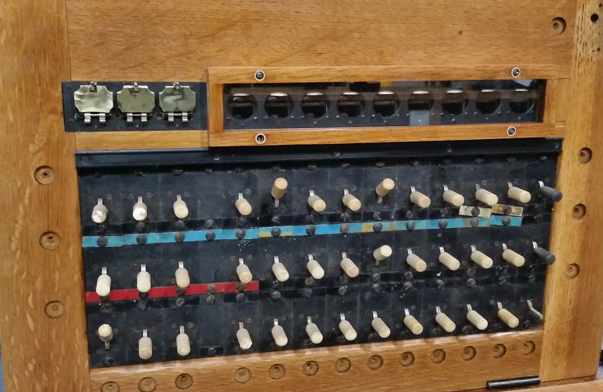
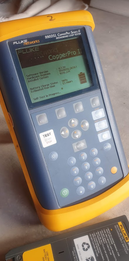
Arguably, the most capable (toolbox-carryable) test set out there is the Fluke 990 CopperPro, combined TDR, Butt Set, Toner, RFL, Noise meter, etc, etc, it’s a really cool gizmo (And probably worthy of a blog post in itself someday).
Alas mine had stopped taking much of a charge, you’d plug it into the charger, and after 20 minutes of use, it’d report low power and shut down.
Sitting on the charger the Fluke would show the red charging light for about 20 minutes, then the charging light would turn off.
If I unplugged and replugged the charger I’d get red charging light for another few minutes, then turn off again.
Naively, I ruled it to be an issue with the battery (Which is close to 10 years old), and ordered a new one.
But with the new battery in hand, the same issue.
Stupidly, it turns out I was using a 15v charger, technically the unit supports a 15v charger, but it seems after a period, the internal voltage regulator overheats and shuts off, meaning the battery never got a good charge.
Swapping it with a 12v charger and I’m charging without issues.
But not before I ended up ordering a new battery, so now with the new battery I’m getting 15 hours of runtime out of a charge, and still squeezing 7 out of 8 year old battery it originally came with.
Dumb mistake but hopefully an easy fix for anyone with the same issue.
Recently I’ve been working on open source Diameter Routing Agent implementations (See my posts on FreeDiameter).
With the hurdles to getting a DRA working with open source software covered, the next step was to get all my Diameter traffic routed via the DRAs, however I soon rediscovered a Kamailio limitation regarding support for Diameter Routing Agents.
You see, when Kamailio’s C Diameter Peer module makes a decision as to where to route a request, it looks for the active Diameter peers, and finds a peer with the suitable Vendor and Application IDs in the supported Applications for the Application needed.
Unfortunately, a DRA typically only advertises support for one application – Relay.
This means if you have everything connected via a DRA, Kamailio’s CDP module doesn’t see the Application / Vendor ID for the Diameter application on the DRA, and doesn’t route the traffic to the DRA.
The fix for this was twofold, the first step was to add some logic into Kamailio to determine if the Relay application was advertised in the Capabilities Exchange Request / Answer of the Diameter Peer.
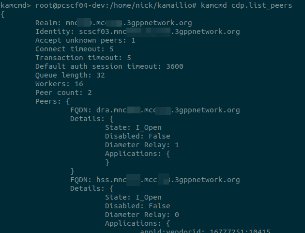
I added the logic to do this and exposed this so you can see if the peer supports Diameter relay when you run “cdp.list_peers”.
With that out of the way, next step was to update the routing logic to not just reject the candidate peer if the Application / Vendor ID for the required application was missing, but to evaluate if the peer supports Diameter Relay, and if it does, keep it in the game.
I added this functionality, and now I’m able to use CDP Peers in Kamailio to allow my P-CSCF, S-CSCF and I-CSCF to route their traffic via a Diameter Routing Agent.
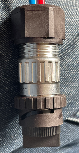
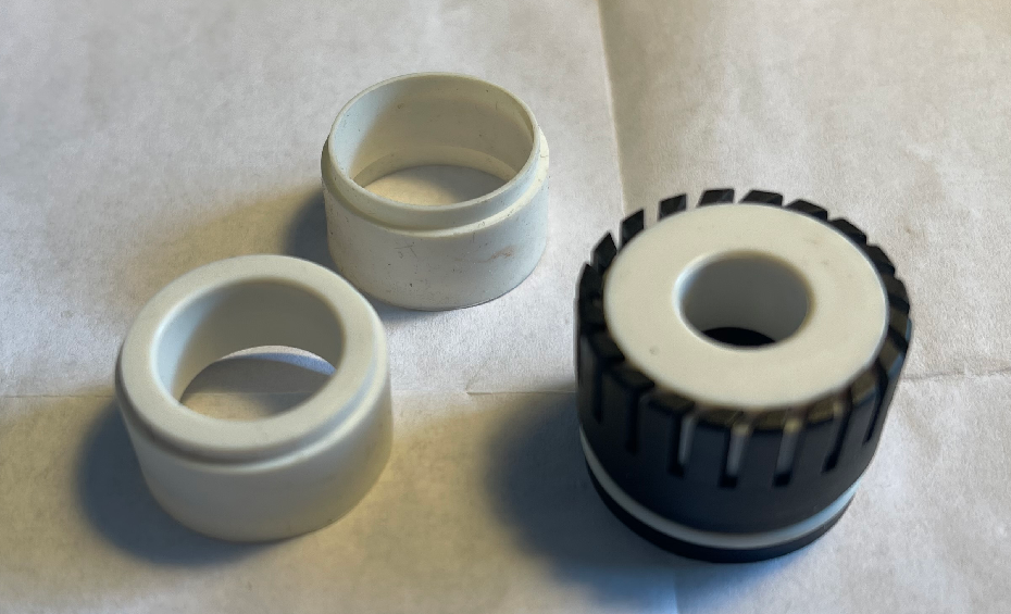
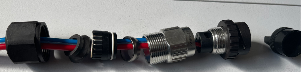
Something that’s kind of great is that the current generation of Ericsson RRUs and Nokia RRUs, use the same power connector – The Amphenol “Amphe-OBTS” series connector.
Construction and wiring of these connectors is the same for both, and with one little trick, we can use the connector for both Ericsson and Nokia RRUs (Airscale and later).
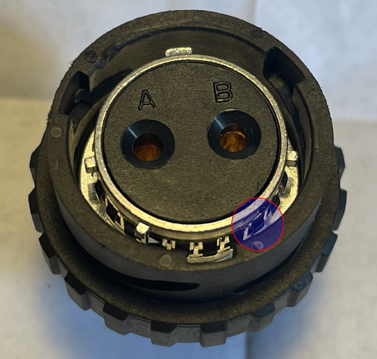
This pin that stops the connector from being “universal” but is easily removed.
The connectors are not quite universal, in order to use it in both you need to knock off a small pin on the connector, I’d suggest doing this before you assemble it, put the connector on it’s back, facing upwards, and hit this with a screwdriver / chisel and it’ll pop off with very little effort.
Assembling the connectors starts by working out the diameter of the grommet you need to fit your cable, the connector comes with the grommet for 9-14mm, but in the bag you’ll usually get grommets for 6-9mm cable and 14-18mm cable.
Grab the correct one for your cable diameter, and pop into the black fingered cage (‘gland adapter’) shown in the bottom right of the below photo.
Grommets and gland adapter
Next we line all the parts up along the cable and screw it all together:
The end-cap is actually very useful for stopping the female end of the connector from spinning when you’re assembling the cable, so don’t throw it away!
Next we’ll need to define our rt_pyform config, this is a super simple 3 line config file that specifies the path of what we’re doing:
DirectoryPath = "."        # Directory to search
ModuleName = "script"      # Name of python file. Note there is no .py extension
FunctionName = "transform" # Python function to call
The DirectoryPath directive specifies where we should search for the Python code, and ModuleName is the name of the Python script, lastly we have FunctionName which is the name of the Python function that does the rewriting.
Now let’s write our Python function for the transformation.
The Python function much have the correct number of parameters, must return a string, and must use the name specified in the config.
The following is an example of a function that prints out all the values it receives:
Note the order of the arguments and that return is of the same type as the AVP value (string).
We can expand upon this and add conditionals, let’s take a look at some more complex examples:
def transform(appId, flags, cmdCode, HBH_ID, E2E_ID, AVP_Code, vendorID, value):
    print('[PYTHON]')
    print(f'|-> appId: {appId}')
    print(f'|-> flags: {hex(flags)}')
    print(f'|-> cmdCode: {cmdCode}')
    print(f'|-> HBH_ID: {hex(HBH_ID)}')
    print(f'|-> E2E_ID: {hex(E2E_ID)}')
    print(f'|-> AVP_Code: {AVP_Code}')
    print(f'|-> vendorID: {vendorID}')
    print(f'|-> value: {value}')
    #IMSI Translation - if App ID = 16777251 and the AVP being evaluated is the Username
    if (int(appId) == 16777251) and int(AVP_Code) == 1:
        print("This is IMSI '" + str(value) + "' - Evaluating transformation")
        print("Original value: " + str(value))
        value = str(value[::-1]).zfill(15)
The above look at if the App ID is S6a, and the AVP being checked is AVP Code 1 (Username / IMSI ) and if so, reverses the username, so IMSI 1234567 becomes 7654321, the zfill is just to pad with leading 0s if required.
Now let’s do another one for a Realm Rewrite:
def transform(appId, flags, cmdCode, HBH_ID, E2E_ID, AVP_Code, vendorID, value):

    #Print Debug Info
    print('[PYTHON]')
    print(f'|-> appId: {appId}')
    print(f'|-> flags: {hex(flags)}')
    print(f'|-> cmdCode: {cmdCode}')
    print(f'|-> HBH_ID: {hex(HBH_ID)}')
    print(f'|-> E2E_ID: {hex(E2E_ID)}')
    print(f'|-> AVP_Code: {AVP_Code}')
    print(f'|-> vendorID: {vendorID}')
    print(f'|-> value: {value}')
    #Realm Translation
    if int(AVP_Code) == 283:
        print("This is Destination Realm '" + str(value) + "' - Evaluating transformation")
    if value == "epc.mnc001.mcc001.3gppnetwork.org":
        new_realm = "epc.mnc999.mcc999.3gppnetwork.org"
        print("translating from " + str(value) + " to " + str(new_realm))
        value = new_realm
    else:
        #If the Realm doesn't match the above conditions, then don't change anything
        print("No modification made to Realm as conditions not met")
    print("Updated Value: " + str(value))
In the above block if the Realm is set to epc.mnc001.mcc001.3gppnetwork.org it is rewritten to epc.mnc999.mcc999.3gppnetwork.org, hopefully you can get a handle on the sorts of transformations we can do with this – We can translate any string type AVPs, which allows for hostname, realm, IMSI, Sh-User-Data, Location-Info, etc, etc, to be rewritten.
NB-IoT introduces support for NIDD – Non-IP Data Delivery (NIDD) which is one of the cool features of NB-IoT that’s gaining more widespread adoption.
Let’s take a deep dive into NIDD.
The case against IP for IoT
In the over 40 years since IP was standardized, we’ve shoehorned many things onto IP, but IP was never designed or optimized for low power, low throughput applications.
For the battery life of an IoT device to be measured in years, it has to be very selective about what power hungry operations it does. Transmitting data over the air is one of the most power-intensive operations an IoT device can perform, so we need to do everything we can to limit how much data is sent, and how frequently.
Use Case – NB-IoT Tap
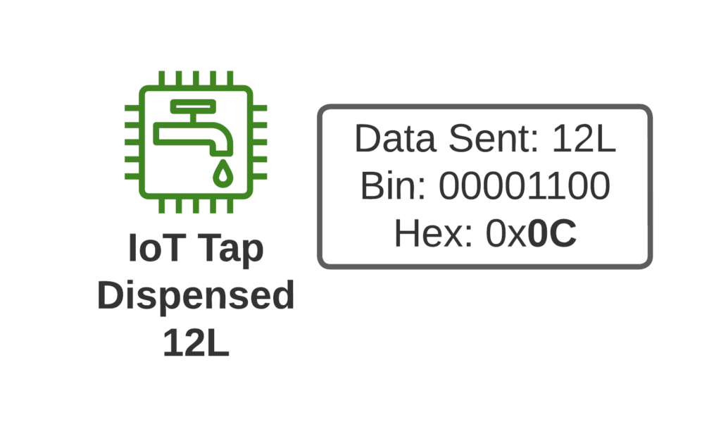
Let’s imagine we’re launching an IoT tap that transmits information about water used, as part of our revolutionary new “Water as a Service” model (WaaS) which removes the capex for residents building their own water treatment plant in their homes, and instead allows dynamic scaling of waterloads as they move to our new opex model.
If I turn on the tap and use 12L of water, when I turn off the tap, our IoT tap encodes the usage onto a single byte and sends the usage information to our rain-cloud service provider.
So we’re not constantly changing the batteries in our taps, we need to send this one byte of data as efficiently as possible, so as to maximize the battery life.
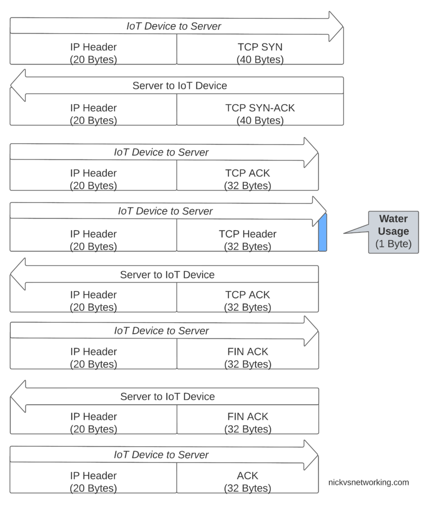
If we were to transport our data on TCP, well we’d need a 3 way handshake and several messages just to transmit the data we want to send.
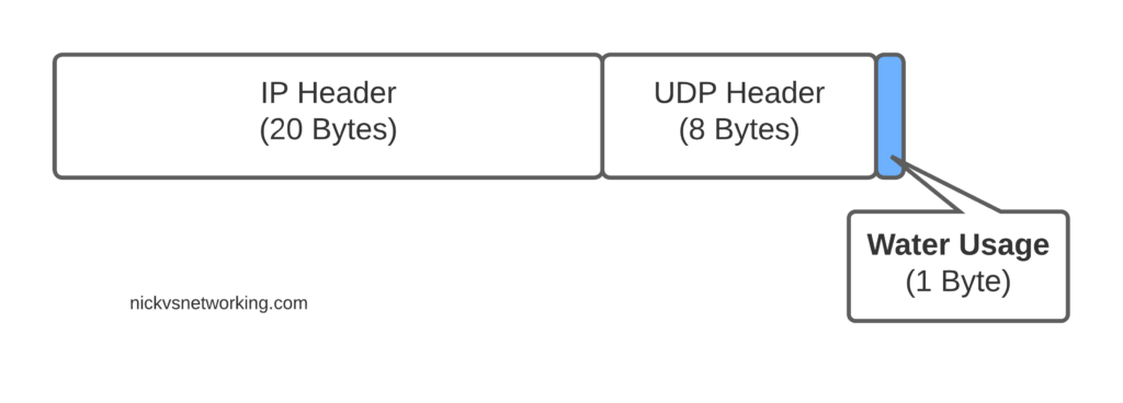
Let’s see how our one byte of data would look if we transported it on TCP.
That sliver of blue in the diagram is our usage component, the rest is overhead used to get it there. Seems wasteful huh?
Sure, TCP isn’t great for this you say, you should use UDP! But even if we moved away from TCP to UDP, we’ve still got the IPv4 header and the UDP header wasting 28 bytes.
For efficiency’s sake (To keep our batteries lasting as long as possible) we want to send as few messages as possible, and where we do have to send messages, keep them very short, so IP is not a great fit here.
Enter NIDD – Non-IP Data Delivery.
Through NIDD we can just send the single hex byte, only be charged for the single hex byte, and only stay transmitting long enough to send this single byte of hex (Plus the NBIoT overheads / headers).
Compared to UDP transport, NIDD provides us a reduction of 28 bytes of overhead for each message, or a 96% reduction in message size, which translates to real power savings for our IoT device.
In summary – the more sending your device has to do, the more battery it consumes. So in a scenario where you’re trying to maximize power efficiency to keep your batter powered device running as long as possible, needing to transmit 28 bytes of wasted data to transport 1 byte of usable data, is a real waste.
Delivering the Payload
NIDD traffic is transported as raw hex data end to end, this means for our 1 byte of water usage data, the device would just send the hex value to be transferred and it’d pop out the other end.
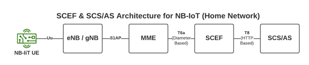
To support this we introduce a new network element called the SCEF –Service Capability Exposure Function.
From a developer’s perspective, the SCEF is the gateway to our IoT devices. Through the RESTful API on the SCEF (T8 API), we can send and receive raw hex data to any of our IoT devices.
When one of our Water-as-a-Service Taps sends usage data as a hex byte, it’s the software talking on the T8 API to the SCEF that receives this data.
Data of course needs to be addressed, so we know where it’s coming from / going to, and T8 handles this, as well as message reliability, etc, etc.
This is a telco blog, so we should probably cover the MME connection, the MME talks via Diameter to the SCEF. In our next post we’ll go into these signaling flows in more detail.
If you’re wondering what the status of Open Source SCEF implementations are, then you may have already guessed I’m working on one!
Hopefully by now you’ve got a bit of an idea of how NIDD works in NB-IoT, and in our next posts we’ll dig deeper into the flows and look at some PCAPs together.