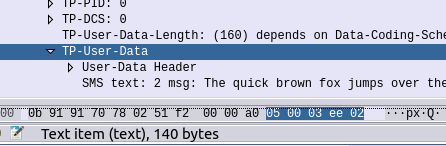
SMS by default uses the GSM-7 bit alphabet, thanks to the fact each letter is only 7 bits long, this means you can cram 160 characters into a 140 byte message body.
However, this 7-bit alphabet is, well, limited, because it’s 7 bits long it means we can only have 128 different combinations of these bits, or to put it another way, with only 128 different unique combinations of these bits, we can only define 128 characters.
You have the standard 26 latin alphabet characters that Sesame Street drilled into you, some characters with accents, digits, and a limited set of symbols.
The GSM 7 bit alphabet does not include is character sets and symbols common for non-English written languages.
Shift Tables
To deal with this 3GPP introduced “National Language Shift Tables”, which are enable a sort of find-and-replace approach to the 7-bit alphabet, where certain characters that are unused in one alphabet, take the value of characters from the local alphabet.
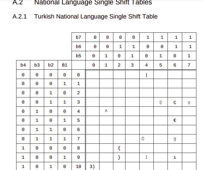
So if you want to send the character Ğ (Found in the Turkish and Azerbaijani alphabets) you’d select the Turkish language Shift table, that replaces the capital G (71) with Ğ.
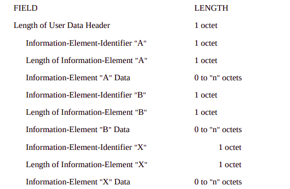
Of course you need to have two things to do this, you need the Language Shift Table to tell you what local-language letters replace what default letters, and a mechanism to state that you’re using a language shift table.
3GPP define the National Language Shift tables in TS 23.038, where you can lookup the character you want to encode, so you know what 7 bit value it uses, for example our character Ğ is 1000111 in the 7-bit alphabet.
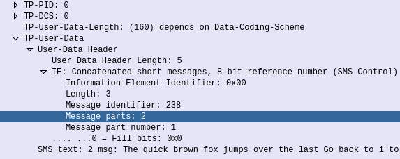
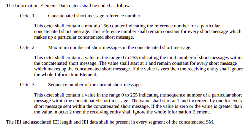
Next we need to indicate that we don’t want 1000111 in the 7-bit alphabet to be rendered as “G”, we want to use the “Turkish National Language Single Shift Table” which will render it as “Ğ”. We do this in the User Data Header of the SMS Body, the same way we’d indicate that an SMS is a concatenated SMS.
But by adding a header in the User Data Header of the SMS Body, we eat into the space we can use to send the message body, with a single User Data Header indicating that the Turkish National Language Single Shift Table is being used, we go from a maximum of 160 characters without the User Data Header, to 134 characters.
I’ve shared a lot more information on the User Data Header in this post on Concatenated SMS, should you be interested.
UCS2 Encoding
So that’s all well and good for other languages that have some overlap in letters, where we can substitute “G” for “Ğ”, but Unicode have 3304 emojis defined at the time of writing.
No matter how many shift tables you define, you’re not going to cover all of these in a 7-bit alphabet.
So all this encoding falls to 💩 when someone adds an Emoji.
The “😀” Emoji, represented as U+1F600 in Unicode, can be encoded as 0xF09F9880 in UTF-8 or 0xD83DDE00 in UTF-16.
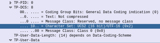
So in 3GPP Networks, when you need more than 128 characters to work with, and when shift tables won’t cut the mustard, you can change the encoding used to use the International Standards Organisations’ “Universal coded character set 2” (UCS-2).
Unfortunately UCS-2 never really took off, but luckily it overlaps with UTF-16 character set, which is a lot more common.
So if you’ve got a “😀” Emoji in your SMS body the encoding of the message will be changed from GSM-7 to use a different encoding -UTF-16 / UCS2.
There’s a catch here, if you’re moving from a 7-bit alphabet to a 16 bit alphabet, you’re going to have a lot less space to work with.
A single SMS contains 1120 bits for the user data (The actual message).
With GSM-7 bit encoding, each letter takes up 7 bits, so 1120÷7 gives us 160 characters.
With UTF-16/UCS2 encoding, each letter takes up 16 bits so 1120÷16 only give us 70 characters.
So what happens next?
Often when Emojis are used, as our message is now limited to 70 characters concatenated messages are used, which takes a further 8 bytes of our message body if concatenated messages are used, further limiting the message length.