To support Dedicated Bearers we first have to have a way of profiling the traffic, to classify the traffic as being the type we want to provide the Dedicated Bearer for.
The first step involves a request from an Application Function (AF) to the PCRF via the Rx interface.
The most common type of AF would be a P-CSCF. When a VoLTE call gets setup the P-CSCF requests that a dedicated bearer be setup for the IP Address and Ports involved in the VoLTE call, to ensure users get the best possible call quality.
But Application Functions aren’t limited to just VoLTE – You could also embed an Application Function into the server for an online game to enable a dedicated bearer for users playing that game, or a sports streaming app that detects when a user starts streaming sports and creates a dedicated bearer for that user to send the traffic down.
The request to setup a dedicated bearer comes in the form of a Diameter request message from the AF, using the Rx reference point, typically from the P-CSCF to the PCRF in the network in an “AA-Request”.
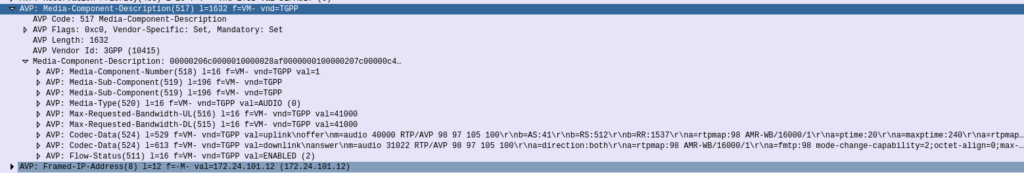
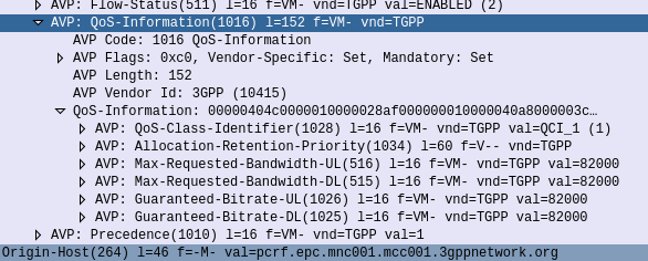
Of main interest in the AA-Request is the Media Component AVP, that contains all the details needed to identify the traffic flow.
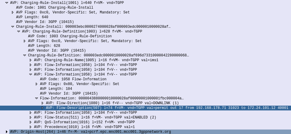
Now our PCRF is in charge of policy, and know which P-GW is serving the required subscriber. So the PCRF takes this information and sends a Gx Re-Auth Request to the PCEF in the P-GW serving the subscriber, with a Charging Rule the PCEF in the P-GW needs to install, to profile and apply QoS to the bearer.
Charging Rule Definition’s Flow-Information AVPs showing the information needed to profile the traffic
The QoS Description AVP defines which QoS parameters (QCI / ARP / Guaranteed & Maximum Bandwidth) should be applied to the traffic that matches the rules we just defined.
QoS Information AVP showing requested QoS Parameters
The P-GW sends back a Gx Re-Auth Answer, and gets to work actually setting up these bearers.
With the rule installed on the PCEF, it’s time to get this new bearer set up on the UE / eNodeB.
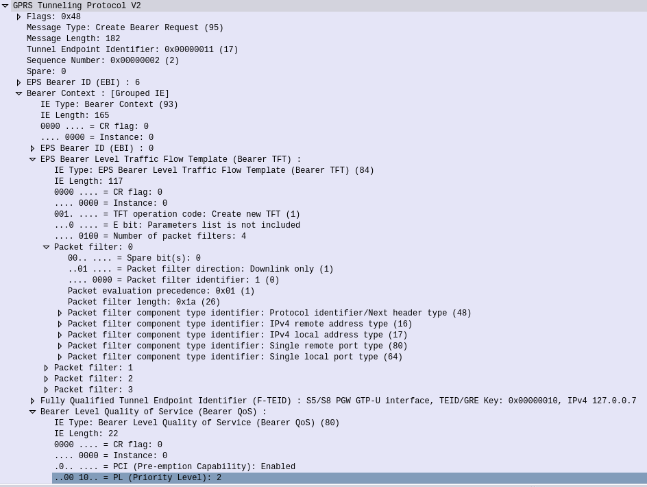
The P-GW sends a GTPv2 “Create Bearer Request” to the S-GW which forwards it onto the MME, to setup / define the Dedicated Bearer to be setup on the eNodeB.
GTPv2 “Create Bearer Request” sent by the P-Gw to the S-GW forwarded from the S-GW to the MME
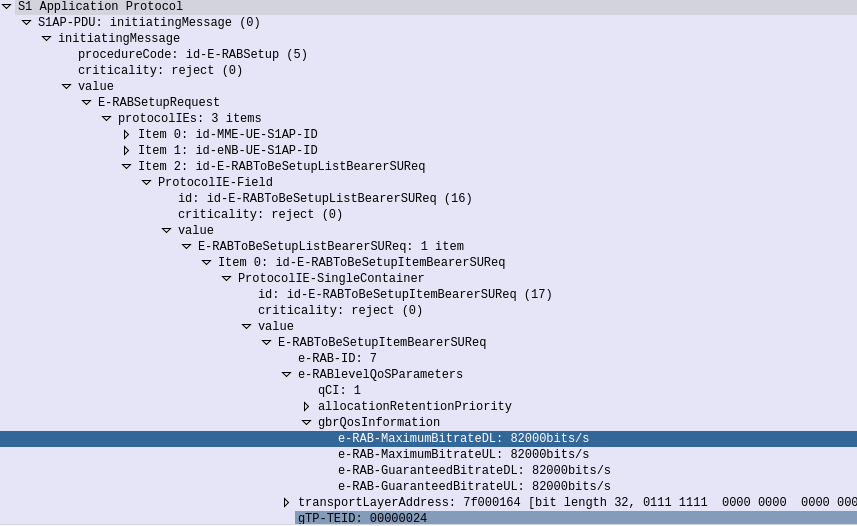
The MME translates this into an S1 “E-RAB Setup Request” which it sends to the eNodeB to setup,
S1 E-RAB Setup request showing the E-RAB to be setup
Assuming the eNodeB has the resources to setup this bearer, it provides the details to the UE and sets up the bearer, sending confirmation back to the MME in the S1 “E-RAB Setup Response” message, which the MME translates back into GTPv2 for a “Create Bearer Response”
All this effort to keep your VoLTE calls sounding great!
The SIP RFC allows for multiple SIP headers to have the same name,
For example, it’s very common to have lots of Via headers present in a request.
In Kamailio, we often may wish to add headers, view the contents of headers and perform an action or re-write headers (Disclaimer about not rewriting Vias as that goes beyond the purview of a SIP Proxy but whatever).
Let’s look at a use case where we have multiple instances of the X-NickTest: header, looking something like this:
INVITE sip:[email protected]:5061 SIP/2.0
X-NickTest: ENTRY ONE
X-NickTest: ENTRY TWO
X-NickTest: ENTRY THREE
...
Let’s look at how we’d access this inside Kamailio.
First, we could just use the psedovariable for header – $hdr()
xlog("Value of X-NickTest is: $hdr(X-NickTest)");
But this would just result in the first entry being printed out:
Value of X-NickTest is: ENTRY ONE
If we know how many instances there are of the header, we can access it by it’s id in the array, for example:
xlog("Value of first X-NickTest is: $hdr(X-NickTest)[0]");
xlog("Value of second X-NickTest is: $hdr(X-NickTest)[1]");
xlog("Value of third  X-NickTest is: $hdr(X-NickTest)[2]");
But we may not know how many to expect either, but we can find out using $hdrc(name) to get the number of headers returned.
xlog("X-NickTest has $hdrc(X-NickTest) entries");
You’re probably seeing where I’m going with this, the next logical step is to loop through them, which we can also do something like this:
$var(i) = 0;
while($var(i) < $hdrc(X-NickTest)) {
         xlog(X-NickTest entry [$var(i)] has value $hdrc(X-NickTest)[$var(i)]);
         $var(i) = $var(i) + 1;
}
Recently I’ve been using Wireguard to fix the things I once used IPsec for.
It was merged into the Mainline Linux kernel late last year, and then in RouterOS 7.0beta7 (2020-Jun-3) the system kernel on RouterOS was upgraded to version 5.6.3 which contains Wireguard support.
Unfortunately this feature is going to stay in the Unstable / Development releases for the time being until a kernel update is done for the stable release to 5.5.3 or higher, but for now I thought I’d try it out.
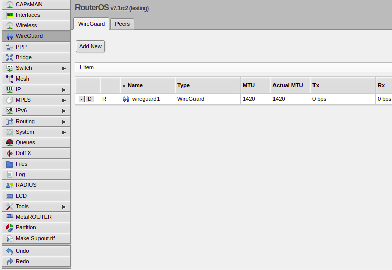
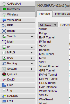
After loading a beta version of the firmware, under Interfaces I have the option to add a Wireguard interface, for clients to connect to my Mikrotik using Wireguard.
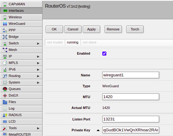
It’s nice and simple to see the public/private key pair (a new key pair is generated for each Wireguard instance which is nifty) that we an use to authenticate / be authenticated.
If we want to configure remote peers, we do this by jumping over to the Wireguard -> Peers tab, allowing us to setup Peers from here.
Obviously routing and firewalls remain to be setup, but I love the simplicity of Wireguard, and in the RouterOS implimentation this is kept.
Through fs_cli you can orignate calls from FreeSWITCH.
At the CLI you can use the originate command to start a call, this can be used for everything from scheduled wake up calls, outbound call centers, to war dialing.
For example, what I’m using:
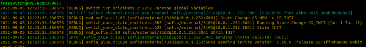
originate sofia/external/[email protected]:5061 61399999995 XML default
originate is the command on the FS_CLI
sofia/external/[email protected]:5061 is the call URL, with the application (I’m using mod_sofia, so sofia), the Sofia Profile (in my case external) and the SIP URI, or, if you have gateways configured, the to URI and the gateway to use.
6139999995 is the Application
XML is the Dialplan to reference
default is the Context to use
But running this on the CLI is only so useful, we can use an ESL socket to use software to connect to FreeSWITCH’s API (Through the same mechanism fs_cli uses) in order to programmatically start calls.
But to do that first we need to expose the ESL API for inbound connections (Clients connecting to FreeSWITCH’s ESL API, which is different to FreeSWITCH connecting to an external ESL Server where FreeSWITCH is the client).
We’ll need to edit the event_socket.conf.xml file to define how this can be accessed:
Obviously you’ll need to secure this appropriately, good long password, and tight ACLs.
You may notice after applying these changes in the config, you’re no longer able to run fs_cli and access FreeSWITCH, this is because FreeSWITCH’s fs_cli tool connects to FreeSWITCH over ESL, and we’ve just changed tha parameters. You should still be able to connect by specifying the IP Address, port and the secret password we set:
This also means we can run fs_cli from other hosts if permitted through the ACLs (kinda handy for managing larger clusters of FreeSWITCH instances).
But now we can also connect a remote ESL client to it to run commands like our Originate command to setup calls, I’m using GreenSwitch with ESL in Python:
import gevent
import greenswitch
import sys
#import Fonedex_TelephonyAPI
#sys.path.append('../WebUI/Flask/')
import uuid

import logging
logging.basicConfig(level=logging.DEBUG)


esl_server_host = "10.0.1.16"
logging.debug("Originating call to " + str(destination) + " from " + str(source))
logging.debug("Routing the call to " + str(dialplan_entry))
fs = greenswitch.InboundESL(host=str(esl_server_host), port=8021, password='yoursecretpassword')
  try:
      fs.connect()
      logging.debug("Connected to ESL server at " + str(esl_server_host))
  except:
      raise SystemError("Failed to connect to ESL Server at " + str(esl_server_host))

r = fs.send('bgapi originate {origination_caller_id_number=' + str(source) + '}sofia/external/' + str(destination) + '@10.0.1.252:5061 default XML')
So I’ve been waxing lyrical about how cool in the NRF is, but what about how it’s secured?
A matchmaking service for service-consuming NFs to find service-producing NFs makes integration between them a doddle, but also opens up all sorts of attack vectors.
Theoretical Nasty Attacks (PoC or GTFO)
Sniffing Signaling Traffic: A malicious actor could register a fake UDR service with a higher priority with the NRF. This would mean UDR service consumers (Like the AUSF or UDM) would send everything to our fake UDR, which could then proxy all the requests to the real UDR which has a lower priority, all while sniffing all the traffic.
Stealing SIM Credentials: Brute forcing the SUPI/IMSI range on a UDR would allow the SIM Card Crypto values (K/OP/Private Keys) to be extracted.
Sniffing User Traffic: A dodgy SMF could select an attacker-controlled / run UPF to sniff all the user traffic that flows through it.
Obviously there’s a lot more scope for attack by putting nefarious data into the NRF, or querying it for data gathering, and I’ll see if I can put together some examples in the future, but you get the idea of the mischief that could be managed through the NRF.
This means it’s pretty important to secure it.
OAuth2
3GPP selected to use common industry standards for HTTP Auth, including OAuth2 (Clearly lessons were learned from COMP128 all those years ago), however OAuth2 is optional, and not integrated as you might expect. There’s a little bit to it, but you can expect to see a post on the topic in the next few weeks.
3GPP Security Recommendations
So how do we secure the NRF from bad actors?
Well, there’s 3 options according to 3GPP:
Option 1 – Mutual TLS
Where the Client (NF) and the Server (NRF) share the same TLS info to communicate.
This is a pretty standard mechanism to use for securing communications, but the reliance on issuing certificates and distributing them is often done poorly and there is no way to ensure the person with the certificate, is the person the certificate was issued to.
3GPP have not specified a mechanism for issuing and securely distributing certificates to NFs.
Option 2 – Network Domain Security (NDS)
Split the network traffic on a logical level (VLANs / VRFs, etc) so only NFs can access the NRF.
Essentially it’s logical network segregation.
Option 3 – Physical Security
Split the network like in NDS but a physical layer, so the physical cables essentially run point-to-point from NF to NRF.
NRF and NF shall authenticate each other during discovery, registration, and access token request. If the PLMN uses protection at the transport layer as described in clause 13.1, authentication provided by the transport layer protection solution shall be used for mutual authentication of the NRF and NF. If the PLMN does not use protection at the transport layer, mutual authentication of NRF and NF may be implicit by NDS/IP or physical security (see clause 13.1). When NRF receives message from unauthenticated NF, NRF shall support error handling, and may send back an error message. The same procedure shall be applied vice versa. After successful authentication between NRF and NF, the NRF shall decide whether the NF is authorized to perform discovery and registration. In the non-roaming scenario, the NRF authorizes the Nnrf_NFDiscovery_Request based on the profile of the expected NF/NF service and the type of the NF service consumer, as described in clause 4.17.4 of TS23.502 [8].In the roaming scenario, the NRF of the NF Service Provider shall authorize the Nnrf_NFDiscovery_Request based on the profile of the expected NF/NF Service, the type of the NF service consumer and the serving network ID. If the NRF finds NF service consumer is not allowed to discover the expected NF instances(s) as described in clause 4.17.4 of TS 23.502[8], NRF shall support error handling, and may send back an error message. NOTE 1: When a NF accesses any services (i.e. register, discover or request access token) provided by the NRF , the OAuth 2.0 access token for authorization between the NF and the NRF is not needed.
TS 133 501 – 13.3.1 Authentication and authorization between network functions and the NRF
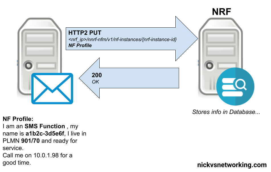
The Network Repository Function plays matchmaker to all the elements in our 5G Core.
For our 5G Service-Based-Architecture (SBA) we use Service Based Interfaces (SBIs) to communicate between Network Functions. Sometimes a Network Function acts as a server for these interfaces (aka “Service Producer”) and sometimes it acts as a client on these interfaces (aka “Service Consumer”).
For service consumers to be able to find service producers (Clients to be able to find servers), we need a directory mechanism for clients to be able to find the servers to serve their needs, this is the role of the NRF.
With every Service Producer registering to the NRF, the NRF has knowledge of all the available Service Producers in the network, so when a Service Consumer NF comes along (Like an AMF looking for UDM), it just queries the NRF to get the details of who can serve it.
Basic Process – NRF Registration
In order to be found, a service producer NF has to register with the NRF, so the NRF has enough info on the service-producer to be able to recommend it to service-consumers.
This is all the basic info, the Service Based Interfaces (SBIs) that this NF serves, the PLMN, and the type of NF.
The NRF then stores this information in a database, ready to be found by SBI Service Consumers.
This is achieved by the Service Producing NF sending a HTTP2 PUT to the NRF, with the message body containing all the particulars about the services it offers.
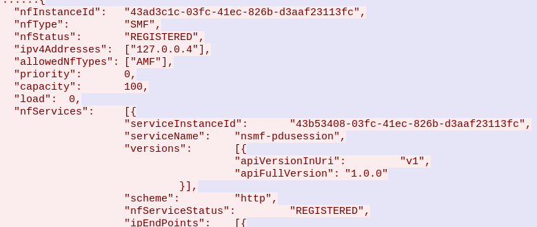
Simplified example of an SMSc registering with the NRF in a 5G Core
Basic Process – NRF Discovery
With an NRF that has a few SBI Service Producers registered in it, we can now start querying it from SBI Service Consumers, to find SBI Service Producers.
The SBI Service Consumer looking for a SBI Service Producer, queries the NRF with a little information about itself, and the SBI Service Producer it’s looking for.
For example a SMF looking for a UDM, sends a request like:
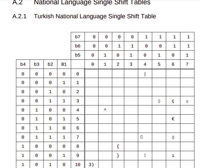
SMS by default uses the GSM-7 bit alphabet, thanks to the fact each letter is only 7 bits long, this means you can cram 160 characters into a 140 byte message body.
However, this 7-bit alphabet is, well, limited, because it’s 7 bits long it means we can only have 128 different combinations of these bits, or to put it another way, with only 128 different unique combinations of these bits, we can only define 128 characters.
You have the standard 26 latin alphabet characters that Sesame Street drilled into you, some characters with accents, digits, and a limited set of symbols.
The GSM 7 bit alphabet does not include is character sets and symbols common for non-English written languages.
Shift Tables
To deal with this 3GPP introduced “National Language Shift Tables”, which are enable a sort of find-and-replace approach to the 7-bit alphabet, where certain characters that are unused in one alphabet, take the value of characters from the local alphabet.
So if you want to send the character Ğ (Found in the Turkish and Azerbaijani alphabets) you’d select the Turkish language Shift table, that replaces the capital G (71) with Ğ.
Of course you need to have two things to do this, you need the Language Shift Table to tell you what local-language letters replace what default letters, and a mechanism to state that you’re using a language shift table.
3GPP define the National Language Shift tables in TS 23.038, where you can lookup the character you want to encode, so you know what 7 bit value it uses, for example our character Ğ is 1000111 in the 7-bit alphabet.
Next we need to indicate that we don’t want 1000111 in the 7-bit alphabet to be rendered as “G”, we want to use the “Turkish National Language Single Shift Table” which will render it as “Ğ”. We do this in the User Data Header of the SMS Body, the same way we’d indicate that an SMS is a concatenated SMS.
But by adding a header in the User Data Header of the SMS Body, we eat into the space we can use to send the message body, with a single User Data Header indicating that the Turkish National Language Single Shift Table is being used, we go from a maximum of 160 characters without the User Data Header, to 134 characters.
I’ve shared a lot more information on the User Data Header in this post on Concatenated SMS, should you be interested.
No matter how many shift tables you define, you’re not going to cover all of these in a 7-bit alphabet.
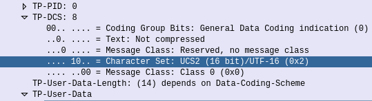
So all this encoding falls to 💩 when someone adds an Emoji.
The “😀” Emoji, represented as U+1F600 in Unicode, can be encoded as 0xF09F9880 in UTF-8 or 0xD83DDE00 in UTF-16.
So in 3GPP Networks, when you need more than 128 characters to work with, and when shift tables won’t cut the mustard, you can change the encoding used to use the International Standards Organisations’ “Universal coded character set 2” (UCS-2).
Unfortunately UCS-2 never really took off, but luckily it overlaps with UTF-16 character set, which is a lot more common.
So if you’ve got a “😀” Emoji in your SMS body the encoding of the message will be changed from GSM-7 to use a different encoding -UTF-16 / UCS2.
SMS Body showing TP-DCS character set is UCS2 / UTF-16 as Emojis are present
There’s a catch here, if you’re moving from a 7-bit alphabet to a 16 bit alphabet, you’re going to have a lot less space to work with.
A single SMS contains 1120 bits for the user data (The actual message).
With GSM-7 bit encoding, each letter takes up 7 bits, so 1120÷7 gives us 160 characters.
With UTF-16/UCS2 encoding, each letter takes up 16 bits so 1120÷16 only give us 70 characters.
So what happens next?
Often when Emojis are used, as our message is now limited to 70 characters concatenated messages are used, which takes a further 8 bytes of our message body if concatenated messages are used, further limiting the message length.
I recently had a bunch of antennas profiles in .msi format, which is the Planet format for storing antenna radiation patterns, but I’m working in Forsk Atoll, so I needed to convert them,
To load these into Atoll, you need to create a .txt file with each of the MSI files in each of the directories, I could do this by hand, but instead I put together a simple Python script you point at the folder full of your MSI files, and it creates the index .txt file containing a list of files, with the directory name.txt, just replace path with the path to your folder full of MSI files,
#Atoll Index Generator
import os
path = "C:\Users\Nick\Desktop\Antennas\ODV-065R15E-G"
antenna_folder = path.split('\\')[-1]
f = open(path + '\\' + 'index_' + str(antenna_folder) + '.txt', 'w+')
files = os.listdir(path)
for individual_file in files:
    if individual_file[-4:] == ".msi":
        print(individual_file)
        f.write(individual_file + "\n")

f.close()
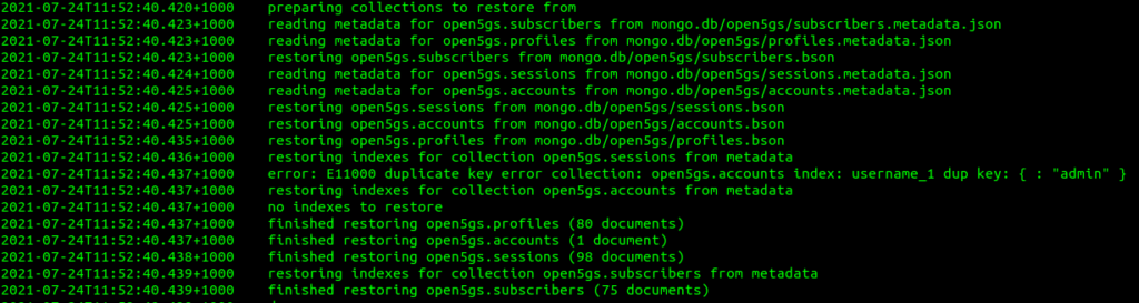
You may find you need to move your Open5GS deployments from one server to another, or split them between servers. This post covers the basics of migrating Open5GS config and data between servers by backing up and restoring it elsewhere.
The Database
Open5GS uses MongoDB as the database for the HSS and PCRF. This database contains all our SDM data, like our SIM Keys, Subscriber profiles, PCC Rules, etc.
Backup Database
To backup the MongoDB database run the below command (It doesn’t need sudo / root to run):
mongodump -o Open5Gs_"`date +"%d-%m-%Y"`"
You should get a directory called Open5Gs_todaysdate, the files in that directory are the output of the MongoDB database.
Restore Database
If you copy the backup we just took (the directory named Open5Gs_todaysdate) to the new server, you can restore the complete database by running:
mongorestore Open5Gs_todaysdate
This restores everything in the database, including profiles and user accounts for the WebUI,
You may instead just restore the Subscribers table, leaving the Profiles and Accounts unchanged with:
The database schema used by Open5GS changed earlier this year, meaning you cannot migrate directly from an old database to a new one without first making a few changes.
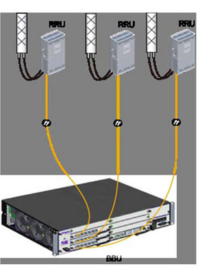
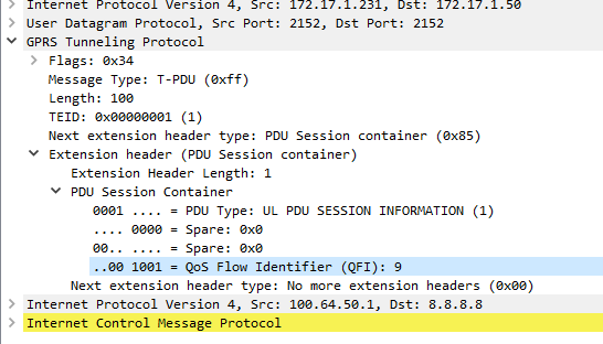
But networks evolve, and 5G Networks required some extensions to GTP to support these on the N9 and N3 reference points. (UPF to UPF and UPF to gNodeB / Access Network).
3GPP TS 38.415 outlines the PDU session user plane protocol used in 5GC.
The Need for GTP Header Extensions
As increasingly complex QoS capabilities are introduced into 5GC, there is a need to signal certain information on a per-packet basis.
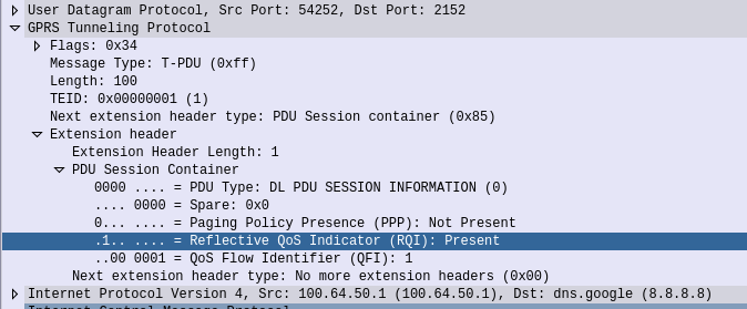
The expansion of QoS in 5GC means the UPF of gNodeB may need to set the QoS Flow Identifier per-packet, include delay measurements or signal that Reflective QoS is being used per packet, for this, you need to extend GTP.
Fortunately GTP has support for Extension Headers and this has been leveraged to add the PDU Session Container in the Extension Header of a GTP packet.
In here you can set on a per packet basis:
QoS Flow Identifier (QFI) – Used to identify the QoS flow to be used (Pretty self explanatory)
Reflective QoS Indicator (RQI) – To indicate reflective QoS is supported for the encapsulated packet
Paging Policy Presence (PPP) – To indicate support for Paging Policy Indicator (PPI)
Paging Policy Indicator (PPI) – Sets parameters of paging policy differentiation to be applied
QoS Monitoring Packet – Indicates packet is used for QoS Monitoring and DL & UL Timestamps to come
UL/DL Sending Time Stamps – 64 bit timestamp generated at the time the UPF or UE encodes the packet
UL/DL Received Time Stamps – 64 bit timestamp generated at the time the UPF or UE received the packet
UL/DL Delay Indicators – Indicates Delay Results to come
UL/DL Delay Results – Delay measurement results
Sequence Number Presence – Indicates if QFI sequence number to come
UL/DL QFI Sequence Number – Sequence number as assigned by the UPF or gNodeB
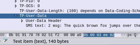
Most people think of 160 characters as the length of an SMS. But the payload is actually 140 bytes, but with better encoding 1 character doesn’t require 1 byte.
The above paragraph is exactly 160 characters. It would fit into a standard SMS.
By using the GSM 7 bit alphabet, you can cram 16 characters into 140 bytes (octets) of space, which is kind of cool.
140 bytes of data containing 160 characters of text
You’d think if you took a 160 character SMS, and concatenated it onto another 160 character SMS, you’d get a total of 320 characters, right (160+160=320)? Alas it’s not that simple.
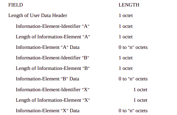
In order to achieve the concatenation of messages in a way that’s transparent to the users (rather than a series of SMSes coming through one-after-the-ther) a User-Data Header (TP-User-Data-Header-Indicator aka TP-UHDI) is added to the TP-User Data of the TPDU (the part that actually contains the user message).
This User-Data Header takes up 7 bytes, which with GSM encoding robs us of 6 characters from the message length. (Not a typo, GSM7 encoding does not mean 1 character = 1 byte, hence we can get 160 characters into 140 bytes of space) So a two SMS concatenated message would only allow 268 characters to be sent (134 characters + 134 characters).
Let’s take a look at this header that’s robbing us of message length, but enabling us to concatenate messages.
For starters, the information about how many parts in the concatenated message, and what part number this one is, is located in the message body, hence robbing us of characters.
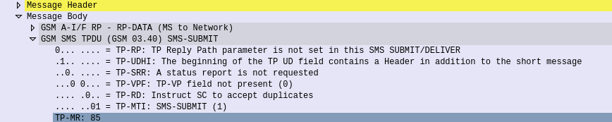
But we only know about the presence of this header being in the message body because the SMS-SUBMIT TPDU has the TP-UDHI flag (TP-User-Data-Header-Indicator) set, so we know the User Data is prefixed with the User-Data-Header.
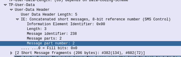
Now if we have a look in the TP-User-Data we can see the User-Data Header, this can actually carry a few different payloads, but in our case, it’s carrying the Concatenated Short Messages IE, which tells us the message identifier (unique per single-but-multi-part message, the number of parts in the message (in this case 2) and the part number this is (part 1 of 2).
First part of a two part SMS
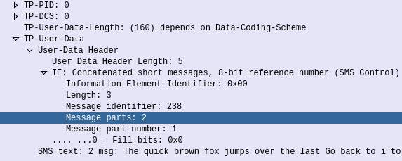
Now the phone has indicated this is a multipart message, the length of the data is still 160, but the length of the actual message is now limited to 134 characters with GSM7 encoding.
The encoding isn’t as bad as you might expect: 1st byte indicates the total length of the User Data Headers (After this the actual user data begins), 2nd byte is the IE identifier, for Concatenated Short Messages, this is 00, 3rd byte is the length of the Concatenated Short Messages IE, 4th byte is the message identifier in hex, 5th byte is the number of message parts in hex (So up to 255 message parts) 6th byte is the message part number, to aid in putting it back together in order.
3GPP TS 23.040 – 9.2.3.24 TP-User Data (TP-UD) – Encoding of User Data Header and generic IEConcatenated short message IE encoding
So what we end up with is a header inside our user payload, advising that this is a concatenated SMS, the message identifier, the number of parts in the message, and the part number of this particular message.
Last part of two part SMS
The SMSc on receipt of these has to spool them back out to the destination with the same message part number, and same headers in place.
The phone receiving the SMS has to wait for all the parts to come through and then reassemble before rendering to the user.
So that’s how concatenated SMS works. While this may seem convoluted and silly in a world where transfering more than 140 bytes of data is trivial, SMS was introduced in the early 1990s, and in theory at least, a user with a phone that supported SMS purchased when SMS was introduced, should still be able to interwork with phones today.
Previous generations of core mobile network, would only allocate a single IP address per UE (Well, two if dual-stack IPv4/IPv6 if you want to be technical). But one of the cool features in 5GC is the support for Framed Routing natively.
You could do this on several EPC platforms on LTE, but it’s support was always a bit shoe-horned in, and the UE was not informed of the framed addresses.
If you’ve worked in a wireline ISP you’re probably familiar with the concept of framed routing already, in short it’s one or more static routes, typically returned from a AAA server (Normally RADIUS) that are then routed to the subscriber.
Each subscriber gets allocated an IP by the network, but other IPs can also be routed to the subscriber, based on the network and CIDR mask.
So let’s say we allocate a public IP of 1.2.3.4/32 to our subscriber, but our subscriber is a fixed-wireless user running a business and they want a extra public IP Addresses.
How do we do this? With Framed Routing.
Now in our UDM we can add a “Framed IP”, and when the SMF sets up a session for our subscriber, the extra networks specified in the framed routes will get routed to that UE.
If we add 203.176.196.0/30 in our UDM for a subscriber, when the subscriber attaches the UPF will be setup to forward traffic to 1.2.3.4/32 and also traffic to 203.176.196.0/30 to the UE.
Update: I previously claimed: Best of all this is signaled to the UE during the attach, so the UE is say a router, it becomes aware of the Framed IPs allocated to it. This is incorrect! Thanks to Anonymous Telco Engineer from an Anonymous Nordic Country for pointing this out, it is not signaled to the UE.
More info in 3GPP TS 23.501 section 5.6.14 Support of Framed Routing.
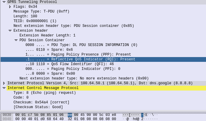
Reflective QoS is a clever new concept introduced in 5G SA networks.
The concept is rather simple, apply QoS in the downlink, and let the UE reply using the QoS in the uplink.
So what is Reflective QoS? If I send an ICMP ping request to a UE with a particular QoS Flow setup on the downlink, if Reflective QoS is enabled, the ICMP reply will have the same QoS applied on the uplink. Simple as that.
The UE looks at the QoS applied on the downlink traffic, and applies the same to the uplink traffic.
Let’s take another example, if a user starts playing an online game, and the traffic to the user (Downlink) has certain QoS parameters set, if Reflective QoS is enabled, the UE builds rules based on the incoming traffic based on the source IP / port / protocol of the traffic received, and the QoS used on the downlink, and applies the same on the uplink.
But actually getting Reflective QoS enabled requires a few more steps…
Reflective QoS is enabled on a per-packet basis, and is indicated by the UPF setting the Reflective QoS Indication (RQI) bit in the encapsulation header next to the QFI (This is set in the GTP header, as an extension header, used on the N3 and N9 reference points).
But before this is honored, a few other parameters have to be setup.
A Reflective QoS Timer (RQ Timer) has to be set, this can be done during the PDU Session Establishment, PDU Session Modification procedure, or set to a default value.
SMF has to set Reflective QoS Attribute (RQA) on the QoS profile for this traffic on the N2 reference point towards gNodeB
SMF must instruct UPF to use uplink reflective QoS by generating a new UL PDR for this SDF via the N4 reference point
When these requirements have been met, the traffic from the UPF to the gNodeB (N3 reference point) has the Reflective QoS Indication (RQI) bit in the encapsulation header, which is encapsulated and signaled down to the UE, which builds a rule based on the received IP source / port / protocol, and sends responses using the same QoS attributes.
Relocating vast numbers of subscriber lines is something to be avoided.
In 1929 Indiana Bell realized they needed a larger telephone exchange (“CO” to use the US term) to meet growing demand, and while there was vacant land around the current building, it wasn’t large enough to build on with the current building slap-dab in the middle of it.
So rather than relocate the subscriber lines to a newly built exchange, they just moved the exchange to the rear of the block, to free up space to build a larger one.
Over a 4 week period engineers shifted the working, 8 story steel and brick telephone exchange, still fully staffed, around to the other side of the block, without any interruptions to the subscribers served from the exchange.
Recently I was working on a project that required Kamailio to constantly re-evaluate something, and generate a UAC request if the condition was met.
There’s a few use cases for this: For example you might want to get Kamailio to constantly check the number of SIP registrations and send an alert if they drop below a certain number. If a subscriber drops out in that their Registration just expires, there’s no SIP message that will come in to tell us, so we’d never be able to trigger something in the normal Kamailio request_route.
Of you might want to continually send a SIP MESSAGE to pop up on someone’s phone to drive them crazy. That’s what this example will focus on.
This is where the rtimer module comes in. You can define the check in a routing block, and then
Like in EPS / LTE, there are two ways to send SMS in Standalone 5G Core networks.
SMS over IMS or SMS over NAS – Both can be used on the same network, or just one, depending on operator preferences.
SMS over IMS in 5G
SMS over IMS uses the IMS network to send SMS. SIP MESSAGE methods are used to deliver SMS between users. While most operators have deployed IMS for 4G/LTE subscribers to use VoLTE some time ago, there are some changes required to the IMS architecture to support VoNR (Voice over New Radio) on the carrier side, and support for VoNR in commercial devices is currently in its early stages. Because of this many 5G devices and networks do not yet support SMS over IMS.
I’ve read in some places that RCS – The GSMA’s Rich Communications Service will replace SMS in 5GC. If this is the case, it reflected in any of the 3GPP standards.
SMS over NAS
To make a voice call on a device or network that does not support VoNR, EPS (VoLTE) fallback is used. This means when making or receiving a call, the UE drops from the 5G RAN to using a 4G (LTE) basd RAN, and then uses VoLTE to make the call the same as it would when connected to 4G (LTE) networks, because it is connected to a 4G network. This works technically, but is not the prefered option as it adds extra signaling and complexity to the network, and delays in the call setup, and it’s expected operators will eventually move to VoNR,but works as a stop-gap measure.
But mobile networks see a lot of SMS traffic. If every time an SMS was sent the UE had to rely on EPS fallback to access IMS, this would see users ping-ponging between 4G and 5G every time they sent or received an SMS.
5GC reintroduces the SMS-over-NAS feature, allowing the SMS messages to be carried over NAS messaging on the N1 interface. Voice calls may still require fallback to EPS (4G) to make calls over VoLTE, but SMS can be carried over NAS messaging, minimizing the amount of Inter-RAT handovers required.
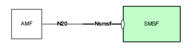
The Nsmsf_SMService
For this a new Service Based Interface is introduced between the AMF and the SMSF (SMS Function, typically built into an SMSc), via the N20 / Nsmsf SBI to offer the Nsmsf_SMService service.
There are 3 operations supported for the Nsmsf_SMService:
Active – Initiated by the AMF – Used to active the SMS service for a given subscriber,
Deactivate – Initiated by the AMF – Used to deactivate the SMS over NAS service for a given subscriber.
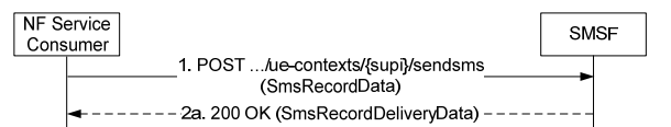
UplinkSMS – Initiated by the AMF to transfer the SMS payload towards the SMSF.
The UplinkSMS is a HTTP post from the AMF with the SUPI in the Request URI and the request body containing a JSON encoded SmsRecordData.
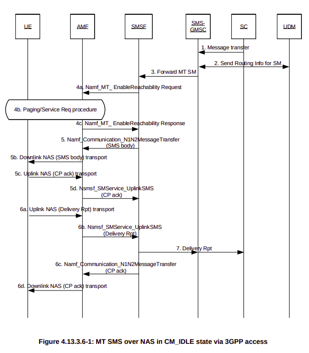
Astute readers may notice that’s all well and good, but that only covers Mobile Originated (MO) SMS, what about Mobile Terminated (MT) SMS?
Well that’s actually handled by a totally different SBI, the Namf_Communication action “N1N2MessageTransfer” is resused for sending MT SMS, as that interface already exists for use by SMF, LMF and PCF, and 5GC attempts to reuse interfaces as much as possible.
There’s no such thing as a free lunch, and 5G is the same – services running through a 5G Standalone core need to be billed.
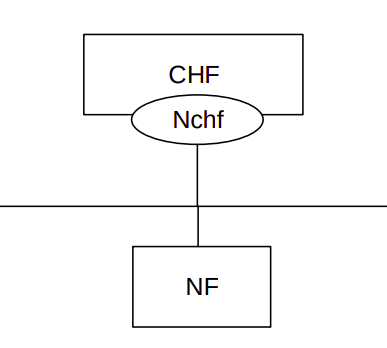
In 5G Core Networks, the SMF (Session Management Function) reaches out to the CHF (Charging Function) to perform online charging, via the Nchf_ConvergedCharging Service Based Interface (aka reference point).
Like in other generations of core mobile networks, Credit Control in 5G networks is based on 3 functions: Requesting a quota for a subscriber from an online charging service, which if granted permits the subscriber to use a certain number of units (in this case data transferred in/out). Just before those units are exhausted sending an update to request more units from the online charging service to allow the service to continue. When the session has ended or or subscriber has disconnected, a termination to inform the online charging service to stop billing and refund any unused credit / units (data).
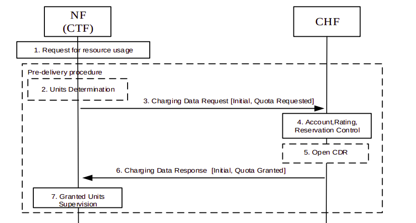
Initial Service Creation (ConvergedCharging_Create)
When the SMF needs to setup a session, (For example when the AMF sends the SMF a Nsmf_PDU_SessionCreate request), the CTF (Charging Trigger Function) built into the SMF sends a Nchf_ ConvergedCharging_Create (Initial, Quota Requested) to the Charging Function (CHF).
Because the Nchf_ConvergedCharging interface is a Service Based Interface this is carried over HTTP, in practice, this means the SMF sends a HTTP post to http://yourchargingfunction/Nchf_ConvergedCharging/v1/chargingdata/
Obviously there’s some additional information to be shared rather than just a HTTP post, so the HTTP post includes the ChargingDataRequest as the Request Body. If you’ve dealt with Diameter Credit Control you may be expecting the ChargingDataRequest information to be a huge jumble of nested AVPs, but it’s actually a fairly short list:
The subscriberIdentifier (SUPI) is included to identify the subscriber so the CHF knows which subscriber to charge
The nfConsumerIdentification identifies the SMF generating the request (The SBI Consumer)
The invocationTimeStamp and invocationSequenceNumber are both pretty self explanatory; the time the request is sent and the sequence number from the SBI consumer
The notifyUri identifies which URI should receive subsequent notifications from the CHF (For example if the CHF wants to terminate the session, the SMF to send that to)
The multipleUnitUsage defines the service-specific parameters for the quota being requested.
The triggers identifies the events that trigger the request
Of those each of the fields should be pretty self explanatory as to their purpose. The multipleUnitUsage data is used like the Service Information AVP in Diameter based Credit Control, in that it defines the specifics of the service we’re requesting a quota for. Inside it contains a mandatory ratingGroup specifying which rating group the CHF should use, and optionally requestedUnit which can define either the amount of service units being requested (For us this is data in/out), or to tell the CHF units are needed. Typically this is used to define the amount of units to be requested.
On the amount of units requested we have a bit of a chicken-and-egg scenario; we don’t know how many units (In our case the units is transferred data in/out) to request, if we request too much we’ll take up all the customer’s credit, potentially prohibiting them from accessing other services, and not enough requested and we’ll constantly slam the CHF with requests for more credit. In practice this value is somewhere between the two, and will vary quite a bit.
Based on the service details the SMF has put in the Nchf_ ConvergedCharging_Create request, the Charging Function (CHF) takes into account the subscriber’s current balance, credit control policies, etc, and uses this to determine if the Subscriber has the required balances to be granted a service, and if so, sends back a 201 CREATED response back to the Nchf_ConvergedCharging_Create request sent by the CTF inside the SMF.
This 201 CREATED response is again fairly clean and simple, the key information is in the multipleQuotaInformation which is nested within the ChargingDataResponse, which contains the finalUnitIndication defining the maximum units to be granted for the session, and the triggers to define when to check in with CHF again, for time, volume and quota thresholds.
And with that, the service is granted, the SMF can instruct the UPF to start allowing traffic through.
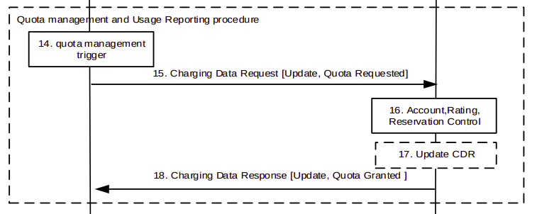
Update (ConvergedCharging_Update)
Once the granted units / quota has been exhausted, the Update (ConvergedCharging_Update) request is used for requesting subsequent usage / quota units. For example our Subscriber has used up all the data initially allocated but is still consuming data, so the SMF sends a Nchf_ConvergedCharging_Update request to request more units, via another HTTP post, to the CHF, with the requested service unit in the request body in the form of ChargingDataRequest as we saw in the initial ConvergedCharging_Create.
If the subscriber still has credit and the CHF is OK to allow their service to continue, the CHF returns a 200 OK with the ChargingDataResponse, again, detailing the units to be granted.
This procedure repeats over and over as the subscriber uses their allocated units.
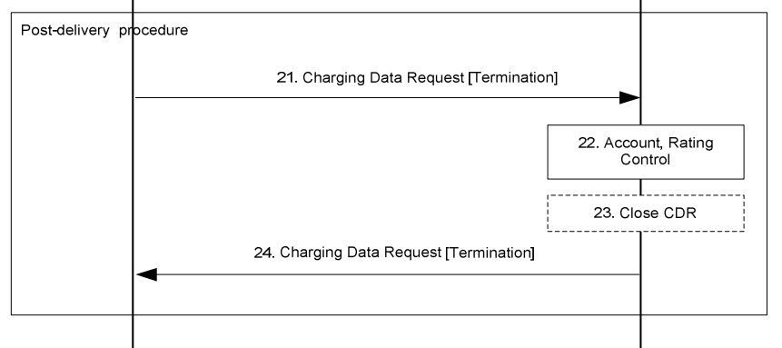
Release (ConvergedCharging_Release)
Eventually when our subscriber disconnects, the SMF will generate a Nchf_ConvergedCharging_Release request, detailing the data the subscriber used in the ChargingDataRequest in the body, to the CHF, so it can refund any unused credits.
The CHF sends back a 204 No Content response, and the procedure is completed.
More Info
If you’ve had experience in Diameter credit control, this simple procedure will be a breath of fresh air, it’s clean and easy to comprehend, If you’d like to learn more the 3GPP specification docs on the topic are clear and comprehensible, I’d suggest:
TS 132 290 – Short overview of charging mechanisms
TS 132 291 – Specifics of the Nchf_ConvergedCharging interface
The common 3GPP charging architecture is specified in TS 32.240
TS 132 291 – Overview of components and SBIs inc Operations
While reading through the 3GPP docs regarding Online Charging, there’s a concept that can be a tad confusing, and that’s the difference between Centralized and Non-Centralized Charging architectures.
The overall purpose of online charging is to answer that deceptively simple question of “does the user have enough credit for this action?”.
In order to answer that question, we need to perform rating and unit determination.
Rating
Rating is just converting connectivity credit units into monetary units.
If you go to the supermarket and they have boxes of Jaffa Cakes at $2.50 each, they have rated a box of Jaffa Cakes at $2.50.
1 Box of Jaffa Cakes rated at $2.50 per box
In a non-snack-cake context, such as 3GPP Online Charging, then we might be talking about data services, for example $1 per GB is a rate for data. Or for a voice calls a cost per minute to call a destination, such as is $0.20 per minute for a local call.
Rating is just working out the cost per connectivity unit (Data or Minutes) into a monetary cost, based on the tariff to be applied to that subscriber.
Unit Determination
The other key piece of information we need is the unit determination which is the calculation of the number of non-monetary units the OCS will offer prior to starting a service, or during a service.
This is done after rating so we can take the amount of credit available to the subscriber and calculate the number of non-monetary units to be offered.
Converting Hard-Currency into Soft-Snacks
In our rating example we rated a box of Jaffa Cakes at $2.50 per box. If I have $10 I can go to the shops and buy 4x boxes of Jaffa cakes at $2.50 per box. The cashier will perform unit determination and determine that at $2.50 per box and my $10, I can have 4 boxes of Jaffa cakes.
Again, steering away from the metaphor of the hungry author, Unit Determination in a 3GPP context could be determining how many minutes of talk time to be granted. Question: At $0.20 per minute to a destination, for a subscriber with a current credit of $20, how many minutes of talk time should they be granted? Answer: 100 minutes ($20 divided by $0.20 per minute is 100 minutes).
Or to put this in a data perspective, Question: Subscriber has $10 in Credit and data is rated at $1 per GB. How many GB of data should the subscriber be allowed to use? Answer: 10GB.
Putting this Together
So now we understand rating (working out the conversion of connectivity units into monetary units) and unit determination (determining the number of non-monetary units to be granted for a given resource), let’s look at the the Centralized and Decentralized Online Charging.
Centralized Rating
In Centralized Rating the CTF (Our P-GW or S-CSCF) only talk about non-monetary units. There’s no talk of money, just of the connectivity units used.
The CTFs don’t know the rating information, they have no idea how much 1GB of data costs to transfer in terms of $$$.
For the CTF in the P-GW/PCEF this means it talks to the OCS in terms of data units (data In/out), not money.
For the CTF in the S-CSCF this means it only ever talks to the OCS in voice units (minutes of talk time), not money.
This means our rates only need to exist in the OCS, not in the CTF in the other network elements. They just talk about units they need.
De-Centralized Rating
In De-Centralized Rating the CTF performs the unit conversion from money into connectivity units. This means the OCS and CTF talk about Money, with the CTF determining from that amount of money granted, what the subscriber can do with that money.
This means the CTF in the S-CSCF needs to have a rating table for all the destinations to determine the cost per minute for a call to a destination.
And the CTF in the P-GW/PCEF has to know the cost per octet transferred across the network for the subscriber.
In previous generations of mobile networks it may have been desirable to perform decentralized rating, as you can spread the load of calculating our the pricing, however today Centralized is the most common way to approach this, as ensuring the correct rates are in each network element is a headache.
Centralized Unit Determination
In Centralized Unit Determination the CTF tells the OCS the type of service in the Credit Control Request (Requested Service Units), and the OCS determines the number of non-monetary units of a certain service the subscriber can consume.
The CTF doesn’t request a value, just tells the OCS the service being requested and subscriber, and the OCS works out the values.
For example, the S-CSCF specifies in the Credit Control Request the destination the caller wishes to reach, and the OCS replies with the amount of talk time it will grant.
Or for a subscriber wishing to use data, the P-GW/PCEF sends a Credit Control Request specifying the service is data, and the OCS responds with how much data the subscriber is entitled to use.
De-Centralized Unit Determination
In De-Centralized Unit Determination, the CTF determines how many units are required to start the service, and requests these units from the OCS in the Credit Control Request.
For a data service,the CTF in the P-GW would determine how many data units it is requesting for a subscriber, and then request that many units from the OCS.
For a voice call a S-CSCF may request an initial call duration, of say 5 minutes, from the OCS. So it provides the information about the destination and the request for 300 seconds of talk time.
Session Charging with Unit Reservation (SCUR)
Arguably the most common online charging scenario is Session Charging with Unit Reservation (SCUR).
SCUR relies on reserving an amount of funds from the subscriber’s balance, so no other services can those funds and translating that into connectivity units (minutes of talk time or data in/out based on the Requested Session Unit) at the start of the session, and then subsequent requests to debit the reserved amount and reserve a new amount, until all the credit is used.
This uses centralized Unit Determination and centralized Rating.
Let’s take a look at how this would look for the CTF in a P-GW/PCEF performing online charging for a subscriber wishing to use data:
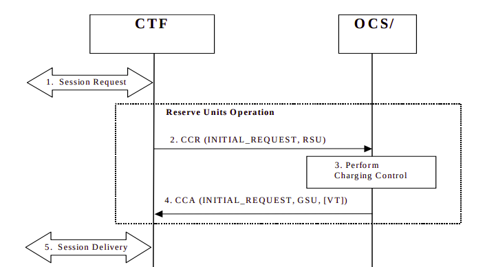
Session Request: The subscriber has attached to the network and is requesting service.
The CTF built into the P-GW/PCEF sends a Credit Control Request: Initial Request (As this subscriber has just attached) to the OCS, with Requested Service Units (RSU) of data in/out to the OCS.
The OCS performs rating and unit determination, and according to it’s credit risk policies, and a whole lot of other factors, comes back with an amount of data the subscriber can use, and reserves the amount from the account. (It’s worth noting at this point that this is not necessarily all of the subscriber’s credit in the form of data, just an amount the OCS is willing to allocate. More data can be requested once this allocated data is used up.)
The OCS sends a Credit Control Answer back to our P-GW/PCEF. This contains the Granted Service Unit (GSU), in our case the GSU is data so defines much data up/down the user can transfer. It also may include a Validity Time (VT), which is the number of seconds the Credit Control Answer is valid for, after it’s expired another Credit Control Request must be sent by the CTF.
Our P-GW/PCEF processes this, starts measuring the data used by the subscriber for reporting later, and sets a timer for the Validity Time to send another CCR at that point. At this stage, our subscriber is able to start using data.
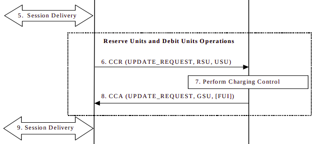
Some time later, either when all the data allocated in the Granted Service Units has been consumed, or when the Validity Time has expired, the CTF in the P-GW/PCEF sends another Credit Control Request:Update, and again includes the RSU (Requested Service Units) as data in/out, and also a USU (Used Service Units) specifying how much data the subscriber has used since the first Credit Control Answer.
The OCS receives this information. It compares the Used Session Units to the Granted Session Units from earlier, and with this is able to determine how much data the subscriber has actually used, and therefore how much credit that equates to, and debit that amount from the account. With this information the OCS can reserve more funds and allocate another GSU (Granted Session Unit) if the subscriber has the required balance. If the subscriber only has a small amount of credit left the FUI (Final Unit Indication AVP) is set to determine this is all the subscriber has left in credit, and if this is exhausted to end the session, rather than sending another Credit Control Request.
The Credit Control Answer with new GSU and the FUI is sent back to the P-GW/PCEF
The P-GW/PCEF allows the session to continue, again monitoring used traffic against the GSU (Granted Session Units).
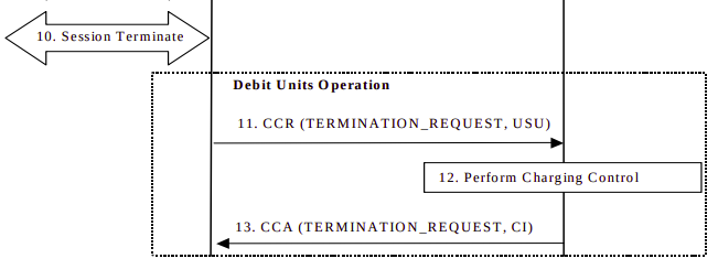
Once the subscriber has used all the data in the Granted Session Units, and as the last CCA included the Final Unit Indicator, the CTF in the P-GW/PCEF knows it can’t just request more credit in the form of a CCR Update, so cuts of the subscribers’s session.
The P-GW/PCEF then sends a Credit Control Request: Termination Request with the final Used Service Units to the OCS.
The OCS debits the used service units from the subscriber’s balance, and refunds any unused credit reservation.
The OCS sends back a Credit Control Answer which may include the CI value for Credit Information, to denote the cost information which may be passed to the subscriber if required.