One of the hyped benefits of a 5G Core Networks is that 5GC can be used for wired networks (think DSL or GPON) – In marketing terms this is called “Wireless Wireline Convergence” (5G WWC) meaning DSL operators, cable operators and fibre network operators can all get in on this sweet 5GC action and use this sexy 5G Core Network tech.
This is something that’s in the standards, and that the big kit vendors are pushing heavily in their marketing materials. But will it take off? And should operators of wireline networks (fixed networks) be looking to embrace 5GC?
Comparing 5GC with current wireline network technologies isn’t comparing apples to apples, it’s apples to oranges, and they’re different fruits.
At its heart, the 3GPP Core Networks (including 5G Core) address one particular use cases of the cellular industry: Subscriber mobility – Allowing a customer to move around the network, being served by different kit (gNodeBs) while keeping the same IP Address.
The most important function of 5GC is subscriber mobility.
This is achieved through the use of encapsulating all the subscriber’s IP data into a GTP (A protocol that’s been around since 2G first added data).
Do I need a 5GC for my Fixed Network?
Wireline networks are fixed. Subscribers don’t constantly move around the network. A GPON customer doesn’t need to move their OLT every 30 minutes to a new location.
Encapsulating a fixed subscriber’s traffic in GTP adds significant processing overhead, for almost no gain – The needs of a wireline network operator, are vastly different to the needs of a cellular core.
Today, you can take a /24 IPv4 block, route it to a DSLAM, OLT or CMTS, and give an IP to 254 customers – No cellular core needed, just a router and your access device and you’re done, and this has been possible for decades. Because there’s no mobility the GTP encapsulation that is the bedrock for cellular, is not needed.
Rather than routing directly to Access Network kit, most fixed operators deploy BRAS systems used for fixed access. Like the cellular packet core, BRAS has been around for a very long time, with a massive install base and a sea of engineering experience in house, it meets the needs of the wireline industry who define its functions and roles along with kit vendors of wireline kit; the fixed industry working groups defined the BRAS in the same way the 3GPP and cellular industry working groups defined 5G Core.
I don’t forsee that we’ll see large scale replacement of BRAS by 5GC, for the same reason a wireless operator won’t replace their mobile core with a BRAS and PPPoE – They’re designed to meet different needs.
All the other features that have been added to the 3GPP Core Network functionality, like limiting speed, guaranteed throughput bearers, 5QI / QCI values, etc, are addons – nice-to-haves. All of these capabilities could be implemented in wireline networks today – if the business case and customer demand was there.
But what about slicing?
With dropping ARPUs across the board, additional services relating to QoS (“Network Slicing”) are being held up as the saving grace of revenues for cellular operators and 5G as a whole, however this has yet to be realized and early indications suggest this is not going to be anywhere near as lucrative as previously hoped.
What about cost savings?
In terms of cost-per-bit of throughput, the existing install base wireline operators have of heavy-metal kit capable of terabit switching and routing has been around for some time in fixed world, and is what most 5G Cores will connect to as their upstream anyway, so there won’t be any significant savings on equipment, power consumption or footprint to be gained.
Fixed networks transport the majority of the world’s data today – Wireline access still accounts for the majority of traffic volumes, so wireline kit handles a higher magnitude of throughput than it’s Packet Core / 5GC cousins already.
Cutting down the number of parts in the network is good though right?
If you’re operating both a Packet Core for Cellular, and a fixed network today, then you might think if you moved from the traditional BRAS architecture fore the wired network to 5GC, you could drop all those pesky routers and switches clogging up your CO, Exchanges and Data Centers.
The problem is that you still need all of those after the 5GC to be able to get the traffic anywhere users want to go. So the 5GC will still need all of that kit, all your border routers and peering routers will remain unchanged, as well as domestic transmission, MPLS and transport.
The parts required for operating fixed networks is actually pretty darn small in comparison to that of 5GC.
TL;DR?
While cellular vendors would love to sell their 5GC platform into fixed operators, the premise that they are willing to replace existing BRAS architectures with 5GC, is as unlikely in my view as 5GC being replaced by BRAS.
In the past I had my iFCs setup to look for the P-Access-Network-Info header to know if the call was coming from the IMS, but it wasn’t foolproof – Fixed line IMS subs didn’t have this header.
If you’ve ever worked in roaming, you’ll probably have had the misfortune of dealing with Transferred Account Procedures aka TAP files.
It’s used for billing a 2G GSM call right up to 5G data usage, if you use a service while roaming, somewhere in the world there’s a TAP file with your usage in it.
A brief history of TAP
TAP was originally specified by the GSMA in 1991 as a standard CDR interchange format between operators, for use in roaming scenarios.
Notice I said GSMA – Not 3GPP – This means there’s no 3GPP TS docs for this, it’s defined by the industry lobby group’s members, rather than the standards body.
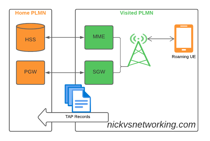
So what does this actually mean? Well, if you’re MNO A and a customer from MNO B roams into your network, all the calls, SMS and data consumed by the roaming subscriber from MNO B will need to be billed to MNO B, by you, MNO A.
If a network operator wants to get paid for traffic used on their network by roaming subscribers, they’d better send out a TAP file to the roamer’s home network.
TAP is the file format generated my MNO A and sent to MNO B, containing all the usage charges that subscribers from MNO B have racked up while roaming into your network.
These are broken down into “Transactions” (CDRs), for events like making a call, connecting a PDN session and consuming data, or sending a text.
In the beginning of time, GSM provided only voice calling service. This meant that the only services a subscriber could consume while roaming was just making/receiving voice calls which were billed at the end of each month. – This meant billing was equally simple, every so often the visisted network would send the TAP files for the voice calls made by subscribers visited other networks, to the home networks, which would markup those charges, and add them onto the monthly invoice for each subscriber who was roaming.
But of course today, calling accounts for a tiny amount of usage on the network, but this happened gradually while passing through the introduction of SMS, CAMEL services, prepaid services, mobile data, etc. For all these services that could be offered, the TAP format had to evolve to handle each of these scenarios.
As we move towards a flat IP architecture, where voice calls and SMS sent while roaming are just data, TAP files for 4G and 5G networks only need to show data transactions, so the call objects, CAMEL parameters and SMS objects are all falling by the wayside.
What’s inside a TAP File
TAP uses the most beloved of formats – ASN1 to encode the data. This means it is strictly formatted and rigidly specified.
Each file contains a Sequence Number which is a monotonically increasing number, which allows the receiver to know if any files have been missed between the file that’s being currently parsed, an the previous file.
They also have a recipient and sender TADIG code, which is a code allocated by GSMA that uniquely identifies the sender and the recipient of the file.
The TAP records exist in one of two common format, Notification Records and transferBatch records.
These files are exchanged between operators, in practice this means “Dumped on an FTP server as agreed between the two”.
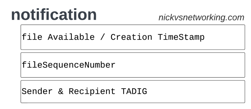
TAP Notification Records
Notifications are the simplest of TAP records and are used when there aren’t any CDRs for roaming events during the time period the TAP file covers.
These are essentially blank TAP files generated by the visited network to let the home network know it’s still there, but there are no roaming subs consuming services in that period.
Notification files are really simple, let’s take a look as one shown as JSON:
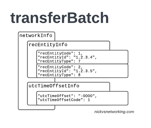
When we have services to bill and records to charge, that’s when instead we generate a transferBatch record.
It looks something like this:
There’s a lot going on in here, so let’s break it down section by section.
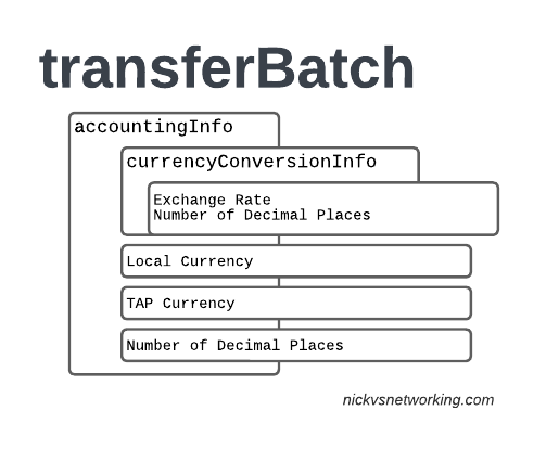
accountingInfo
The accountingInfo section specifies the currency, exchange rate parameters.
Keep in mind a TAP record generated by an operator in the US, would use USD, while the receiver of the file may be a European MNO dealing in EUR.
This gets even more complicated if you’re dealing with more obscure currencies where an intermediary currency is used, that’s where we bring in SDRs (“Special Drawing Right”) that map to the dollar value to be charged, kinda – the roaming agreement defines how many SDRs are in a dollar, in the example below we’re not using any, but you do see it.
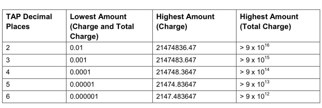
When it comes to numbers and decimal places, TAP doesn’t exactly make it easy.
Significant Digits are defined by counting the first number before the decimal point and all the numbers to the right of the decimal point, so for example the number 1.234 would be 4 significant digits (1 digit before the decimal point and 3 digits after it).
Decimal Places are not actually supported for the Value fields in the TAP file. This is tricky because especially today when roaming tariffs are quite low, these values can be quite small, and we need to represent them as an integer number. TAP defines decimal places as the number of digits after the decimal place.
When it comes to the maximum number of decimal places, this actually impacts the maximum number we can store in the field – as ASN1 strictly enforce what we put in it.
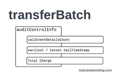
The auditControlInfo section contains the number of CDRs (callEventDetailsCount) contained in the TAP file, the timestamp of the first and last CDR in the file, the total charge and any tax charged.
All of the currency information was provided in the accountingInfo so this is just giving us our totals.
A CDR has 30 days from the time it was generated / service consumed by the roamer, to be baked into a TAP file. After this we can no longer charge for it, so it’s important that the earliestCallTimeStamp is not more than 30 days before the fileCreationTimeStamp seen in batchControlInfo.
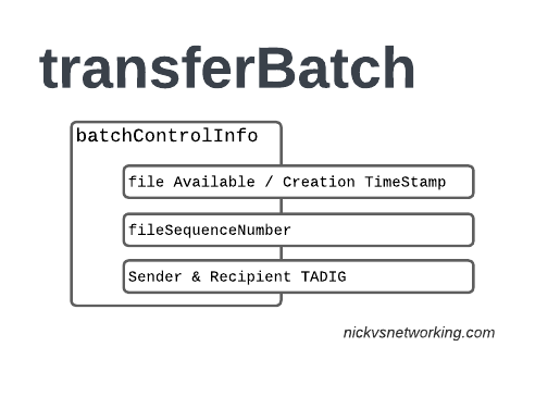
batchControlInfo
The batchControlInfo section specifies the time the TAP file became available for transfer, the time the file was created (usually the same), the sequence number and the sender / recipient TADIG codes.
As mentioned earlier, we track sequence number so the receiver can know if a TAP file has been missed; for example if you’ve got TAP file 1 and TAP file 3 comes in, you can determine you’ve missed TAP file 2.
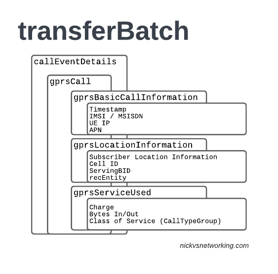
Now we’re getting to the meat & potatoes of our TAP record, the CDRs themselves.
In LTE networks these are just records of data consumption, so let’s take a look inside the gprsCall records under callEventDetails:
In the gprsBasicCallInformation we’ve got as the name suggests the basic info about the data usage event. The time when the session started, the charging ID, the IMSI and the MSISDN of the subscriber to charge, along with their IP and the APN used.
Next up we have the gprsLocationInformation – rates and tariffs may be set based on the location of the subscriber, so we need to identify the area the sub was using the services to select correct tariff / rate for traffic in this destination.
The recEntity is the index number of the SGW / PGW used for the transaction (more on that later).
Next we have the gprsServiceUsed which, again as the name suggests, details the services used and the charge.
chargeDetailList contains the charged data (Made up of dataVolumeIncoming + dataVolumeOutgoing) and the cost.
The chargeableUnits indicates the actual data consumed, however most roaming agreements will standardise on some level of rounding, for example rounding up to the nearest Kilobyte (1024 bytes), so while a sub may consume 1025 bytes of data, they’d be billed for 2045 bytes of data. The data consumed is indicated in the chargeableUnits which indicates how much data was actually consumed, before any rounding policies where applied, while the amount that is actually charged (When taking into account rounding policies) isindicated inside Charged Units.
In the example below data usage is rounded up to the nearest 1024 bytes, 134390 bytes rounds up to the nearest 1024 gives you 135168 bytes.
As this is data we’re talking bytes, but not all bytes are created equal!
VoLTE traffic, using a QCI1 bearer is more valuable than QCI 9 cat videos, and TAP records take this into account in the Call Type Groups, each of which has a different price – Call Type Level 1 indicates the type of traffic, for S8 Home Routed LTE Traffic this is 10 (HGGSN/HP-GW), while Call Type Level 2 indicates the type of traffic as mapped to QCI values:
So Call Type Level 2 set to 20 indicates that this is “20 Unspecified/default LTE QCIs”, and Call Type Level 3 can be set to any value based on a defined inter-operator tariff.
recEntityType 7 means a PGW and contains the IP of the PGW in the Home PLMN, while recEntityType 8 means SGW and is the SGW in the Visited PLMN.
So this means if we reference recEntityCode 2 in a gprsCall, that we’re referring to an SGW at 1.2.3.5.
Lastly also got the utcTimeOffsetInfo to indicate the timezones used and assign a unique code to it.
Using the Records
We as humans? These records aren’t meant for us.
They’re designed to be generated by the Visited PLMN and sent to to the home PLMN, which ingests it and pays the amount specified in the time agreed.
Generally this is an FTP server that the TAP records get dumped into, and an automated bank transfer job based on the totals for the TAP records.
Testing of the TAP records is called “TADIG Testing” and it’s something we’ll go into another day, but in essence it’s validating that the output and contents of the files meet what both operators think is the contract pricing and specifications.
So that’s it! That’s what’s in a TAP record, what it does and how we use it!
GSMA are introducing BCE – Billing & Charging Evolution, a new standard, designed to last for the next 30+ years like TAP has. It’s still in its early days, but that’s the direction the GSMA has indicated it would like to go.
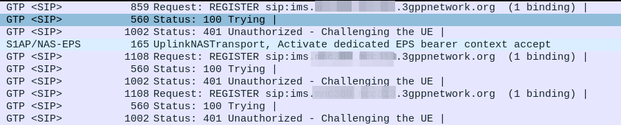
Everything was working on the IMS, then I go to bed, the next morning I fire up the test device and it just won’t authenticate to the IMS – The S-CSCF generated a 401 in response to the REGISTER, but the next REGISTER wouldn’t pass.
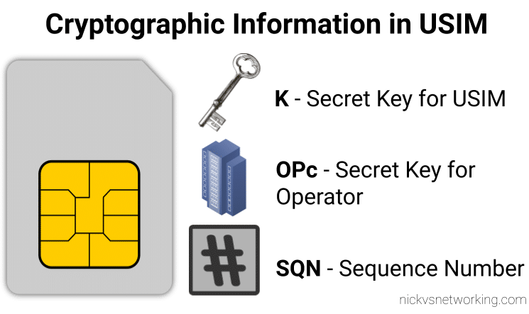
When we generate the vectors (for IMS auth and standard auth) one of the inputs to generate the vectors is the Sequence Number or SQN.
This SQN ticks over like an odometer for the number of times the SIM / HSS authentication process has been performed.
There is some leeway in the SQN – It may not always match between the SIM and the HSS and that’s to be expected. When the MME sends an Authentication-Information-Request it can ask for multiple vectors so it’s got some in reserve for the next time the subscriber attaches, and that’s allowed.
But there are limits to how far out our SQN can be, and for good reason – One of the key purposes for the SQN is to protect against replay attacks, where the same vector is replayed to the UE. So the SQN on the HSS can be ahead of the SIM (within reason), but it can’t be behind – Odometers don’t go backwards.
So the issue was with the SQN on the SIM being out of Sync with the SQN in the IMS, how do we know this is the case, and how do we fix this?
Well there is a resync mechanism so the SIM can securely tell the HSS what the current SQN it is using, so the HSS can update it’s SQN.
When verifying the AUTN, the client may detect that the sequence numbers between the client and the server have fallen out of sync. In this case, the client produces a synchronization parameter AUTS, using the shared secret K and the client sequence number SQN. The AUTS parameter is delivered to the network in the authentication response, and the authentication can be tried again based on authentication vectors generated with the synchronized sequence number.
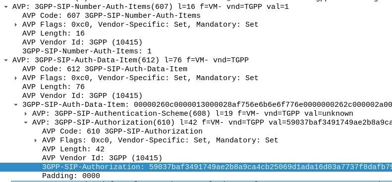
In our example we can tell the sub is out of sync as in our Multimedia Authentication Request we see the SIP-Authorization AVP, which contains the AUTS (client synchronization parameter) which the SIM generated and the UE sent back to the S-CSCF. Our HSS can use the AUTS value to determine the correct SQN.
SIP-Authorization AVP in the Multimedia Authentication Request means the SQN is out of Sync and this AVP contains the RAND and AUTN required to Resync
Note: The SIP-Authorization AVP actually contains both the RAND and the AUTN concatenated together, so in the above example the first 32 bytes are the AUTN value, and the last 32 bytes are the RAND value.
So the HSS gets the AUTS and from it is able to calculate the correct SQN to use.
Then the HSS just generates a new Multimedia Authentication Answer with a new vector using the correct SQN, sends it back to the IMS and presto, the UE can respond to the challenge normally.
Misunderstood, under appreciated and more capable than people give it credit for, is our PCRF.
But what does it do?
Most folks describe the PCRF in hand wavy-terms – “it does policy and charging” is the answer you’ll get, but that doesn’t really tell you anything.
So let’s answer it in a way that hopefully makes some practical sense, starting with the acronym “PCRF” itself, it stands for Policy and Charging Rules Function, which is kind of two functions, one for policy and one for rules, so let’s take a look at both.
Policy
In cellular world, as in law, policy is the rules.
For us some examples of policy could be a “fair use policy” to limit customer usage to acceptable levels, but it can also be promotional packages, services like “free Spotify” packages, “Voice call priority” or “unmetered access to Nick’s Blog and maximum priority” packages, can be offered to customers.
All of these are examples of policy, and to make them work we need to target which subscribers and traffic we want to apply the policy to, and then apply the policy.
Charging Rules
Charging Rules are where the policy actually gets applied and the magic happens.
It’s where we take our policy and turn it into actionable stuff for the cellular world.
Let’s take an example of “unmetered access to Nick’s Blog and maximum priority” as something we want to offer in all our cellular plans, to provide access that doesn’t come out of your regular usage, as well as provide QCI 5 (Highest non dedicated QoS) to this traffic.
To achieve this we need to do 3 things:
Profile the traffic going to this website (so we capture this traffic and not regular other internet traffic)
Charge it differently – So it’s not coming from the subscriber’s regular balance
Up the QoS (QCI) on this traffic to ensure it’s high priority compared to the other traffic on the network
So how do we do that?
Profiling Traffic
So the first step we need to take in providing free access to this website is to filter out traffic to this website, from the traffic not going to this website.
Let’s imagine that this website is hosted on a single machine with the IP 1.2.3.4, and it serves traffic on TCP port 443. This is where IPFilterRules (aka TFTs or “Traffic Flow Templates”) and the Flow-Description AVP come into play. We’ve covered this in the past here, but let’s recap:
IPFilterRules are defined in the Diameter Base Protocol (IETF RFC 6733), where we can learn the basics of encoding them,
They take the format:
action dir proto from src to dst
The action is fairly simple, for all our Dedicated Bearer needs, and the Flow-Description AVP, the action is going to be permit. We’re not blocking here.
The direction (dir) in our case is either in or out, from the perspective of the UE.
Next up is the protocol number (proto), as defined by IANA, but chances are you’ll be using 17 (UDP) or 6 (TCP).
The from value is followed by an IP address with an optional subnet mask in CIDR format, for example from 10.45.0.0/16would match everything in the 10.45.0.0/16 network.
Following from you can also specify the port you want the rule to apply to, or, a range of ports.
Like the from, the tois encoded in the same way, with either a single IP, or a subnet, and optional ports specified.
And that’s it!
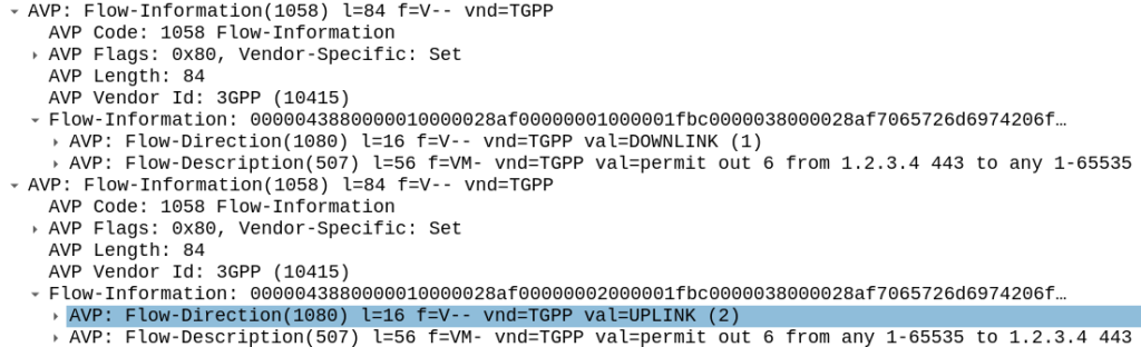
So let’s create a rule that matches all traffic to our website hosted on 1.2.3.4 TCP port 443,
permit out 6 from 1.2.3.4 443 to any 1-65535
permit out 6 from any 1-65535 to 1.2.3.4 443
All this info gets put into the Flow-Information AVPs:
With the above, any traffic going to/from 1.23.4 on port 443, will match this rule (unless there’s another rule with a higher precedence value).
Charging Actions
So with our traffic profiled, the next question is what actions are we going to take, well there’s two, we’re going to provide unmetered access to the profiled traffic, and we’re going to use QCI 4 for the traffic (because you’ll need a guaranteed bit rate bearer to access!).
Charging-Group for Profiled Traffic
To allow for Zero Rating for traffic matching this rule, we’ll need to use a different Rating Group.
Let’s imagine our default rating group for data is 10000, then any normal traffic going to the OCS will use rating group 10000, and the OCS will apply the specific rates and policies based on that.
Rating Groups are defined in the OCS, and dictate what rates get applied to what Rating Groups.
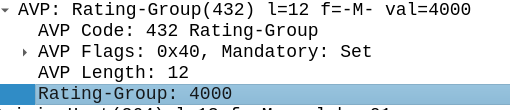
For us, our default rating group will be charged at the normal rates, but we can define a rating group value of 4000, and set the OCS to provide unlimited traffic to any Credit-Control-Requests that come in with Rating Group 4000.
This is how operators provide services like “Unlimited Facebook” for example, a Charging Rule matches the traffic to Facebook based on TFTs, and then the Rating Group is set differently to the default rating group, and the OCS just allows all traffic on that rating group, regardless of how much is consumed.
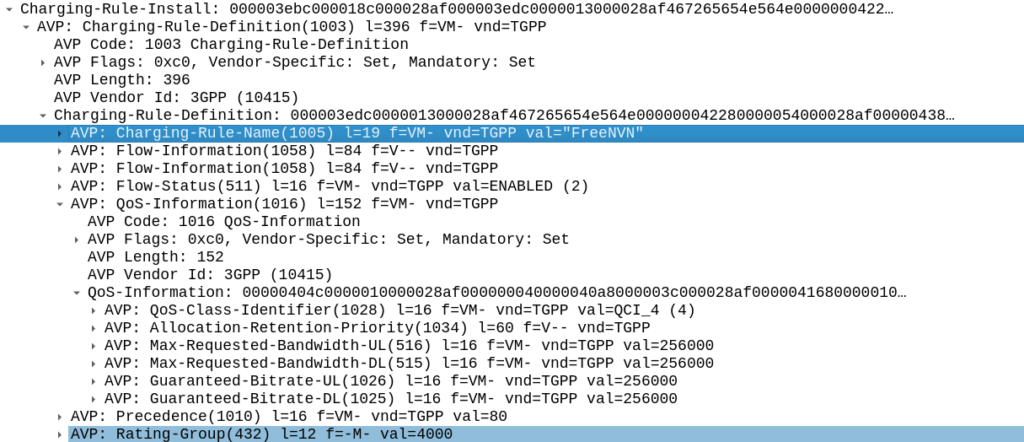
Inside our Charging-Rule-Definition, we populate the Rating-Group AVP to define what Rating Group we’re going to use.
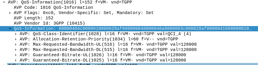
Setting QoS for Profiled Traffic
The QoS Description AVP defines which QoS parameters (QCI / ARP / Guaranteed & Maximum Bandwidth) should be applied to the traffic that matches the rules we just defined.
As mentioned at the start, we’ll use QCI 4 for this traffic, and allocate MBR/GBR values for this traffic.
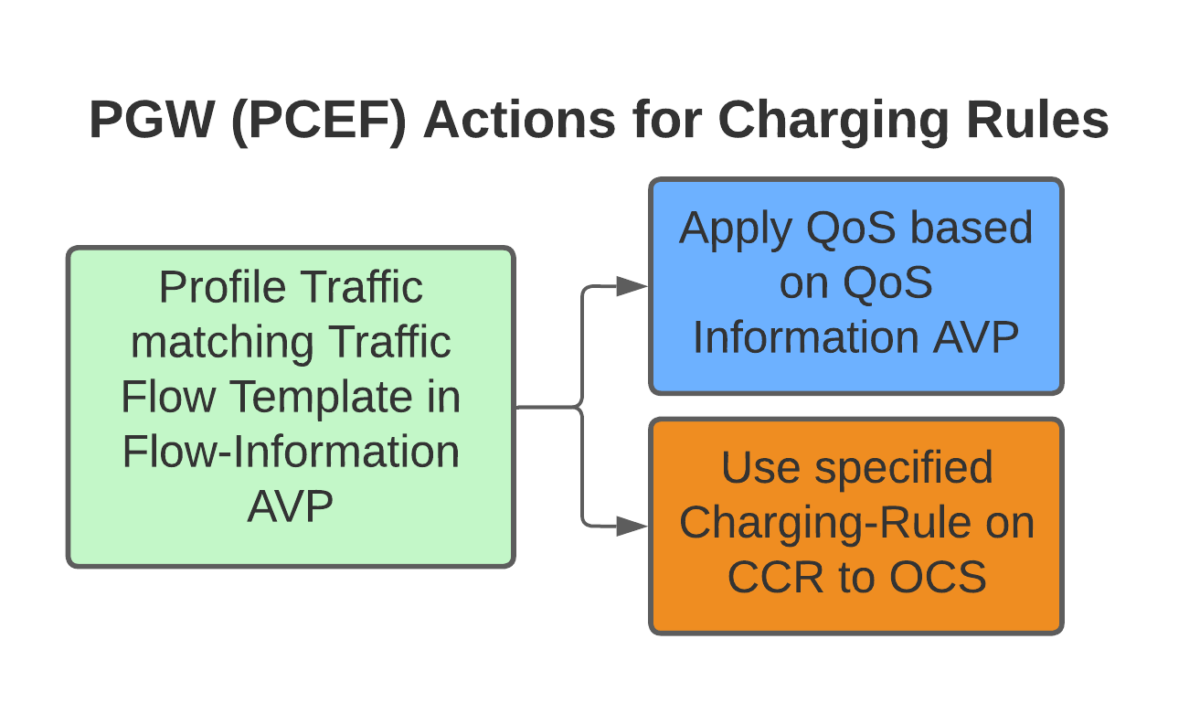
Putting it Together – The Charging Rule
So with our TFTs defined to match the traffic, our Rating Group to charge the traffic and our QoS to apply to the traffic, we’re ready to put the whole thing together.
So here it is, our “Free NVN” rule:
I’ve attached a PCAP of the flow to this post.
In our next post we’ll talk about how the PGW handles the installation of this rule.
Recently I’ve been working on open source Diameter Routing Agent implementations (See my posts on FreeDiameter).
With the hurdles to getting a DRA working with open source software covered, the next step was to get all my Diameter traffic routed via the DRAs, however I soon rediscovered a Kamailio limitation regarding support for Diameter Routing Agents.
You see, when Kamailio’s C Diameter Peer module makes a decision as to where to route a request, it looks for the active Diameter peers, and finds a peer with the suitable Vendor and Application IDs in the supported Applications for the Application needed.
Unfortunately, a DRA typically only advertises support for one application – Relay.
This means if you have everything connected via a DRA, Kamailio’s CDP module doesn’t see the Application / Vendor ID for the Diameter application on the DRA, and doesn’t route the traffic to the DRA.
The fix for this was twofold, the first step was to add some logic into Kamailio to determine if the Relay application was advertised in the Capabilities Exchange Request / Answer of the Diameter Peer.
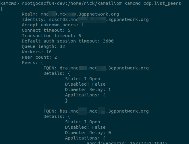
I added the logic to do this and exposed this so you can see if the peer supports Diameter relay when you run “cdp.list_peers”.
With that out of the way, next step was to update the routing logic to not just reject the candidate peer if the Application / Vendor ID for the required application was missing, but to evaluate if the peer supports Diameter Relay, and if it does, keep it in the game.
I added this functionality, and now I’m able to use CDP Peers in Kamailio to allow my P-CSCF, S-CSCF and I-CSCF to route their traffic via a Diameter Routing Agent.
NB-IoT introduces support for NIDD – Non-IP Data Delivery (NIDD) which is one of the cool features of NB-IoT that’s gaining more widespread adoption.
Let’s take a deep dive into NIDD.
The case against IP for IoT
In the over 40 years since IP was standardized, we’ve shoehorned many things onto IP, but IP was never designed or optimized for low power, low throughput applications.
For the battery life of an IoT device to be measured in years, it has to be very selective about what power hungry operations it does. Transmitting data over the air is one of the most power-intensive operations an IoT device can perform, so we need to do everything we can to limit how much data is sent, and how frequently.
Use Case – NB-IoT Tap
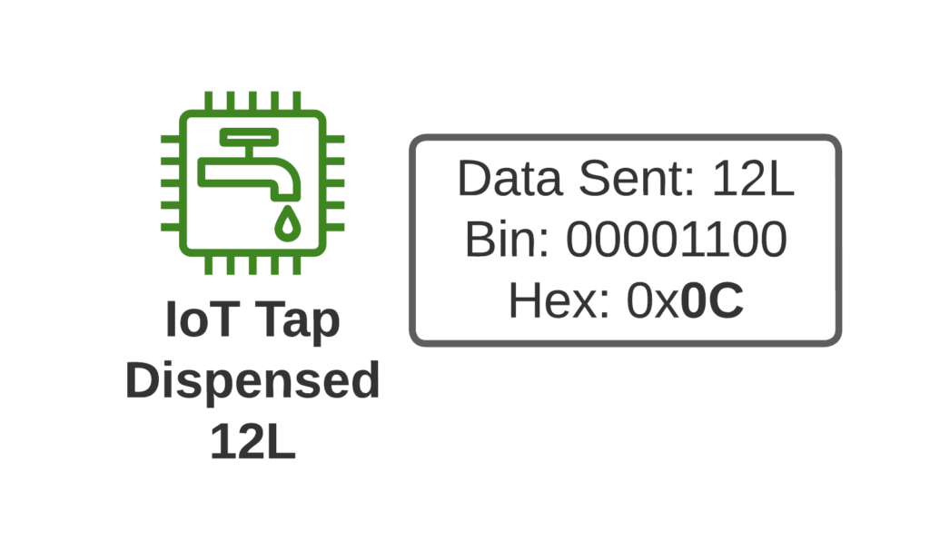
Let’s imagine we’re launching an IoT tap that transmits information about water used, as part of our revolutionary new “Water as a Service” model (WaaS) which removes the capex for residents building their own water treatment plant in their homes, and instead allows dynamic scaling of waterloads as they move to our new opex model.
If I turn on the tap and use 12L of water, when I turn off the tap, our IoT tap encodes the usage onto a single byte and sends the usage information to our rain-cloud service provider.
So we’re not constantly changing the batteries in our taps, we need to send this one byte of data as efficiently as possible, so as to maximize the battery life.
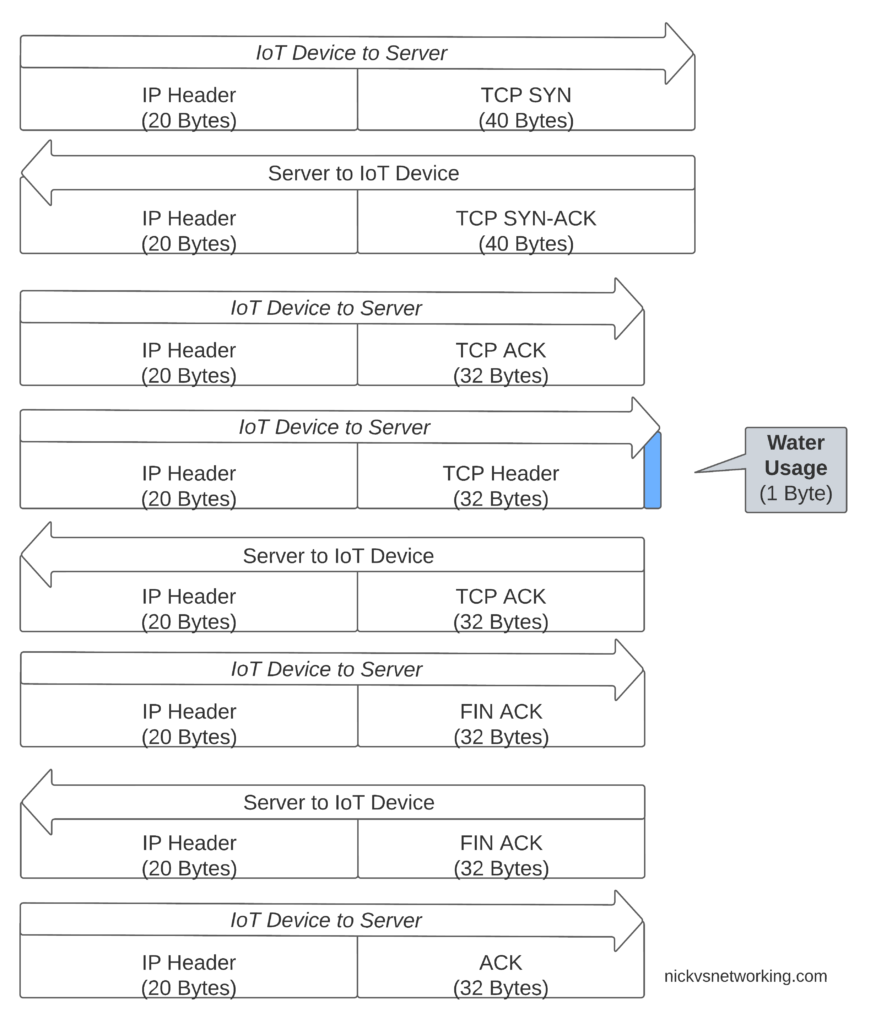
If we were to transport our data on TCP, well we’d need a 3 way handshake and several messages just to transmit the data we want to send.
Let’s see how our one byte of data would look if we transported it on TCP.
That sliver of blue in the diagram is our usage component, the rest is overhead used to get it there. Seems wasteful huh?
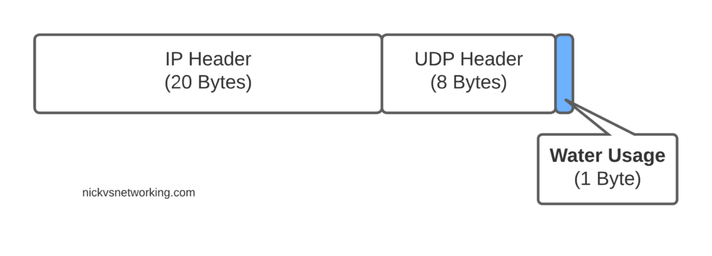
Sure, TCP isn’t great for this you say, you should use UDP! But even if we moved away from TCP to UDP, we’ve still got the IPv4 header and the UDP header wasting 28 bytes.
For efficiency’s sake (To keep our batteries lasting as long as possible) we want to send as few messages as possible, and where we do have to send messages, keep them very short, so IP is not a great fit here.
Enter NIDD – Non-IP Data Delivery.
Through NIDD we can just send the single hex byte, only be charged for the single hex byte, and only stay transmitting long enough to send this single byte of hex (Plus the NBIoT overheads / headers).
Compared to UDP transport, NIDD provides us a reduction of 28 bytes of overhead for each message, or a 96% reduction in message size, which translates to real power savings for our IoT device.
In summary – the more sending your device has to do, the more battery it consumes. So in a scenario where you’re trying to maximize power efficiency to keep your batter powered device running as long as possible, needing to transmit 28 bytes of wasted data to transport 1 byte of usable data, is a real waste.
Delivering the Payload
NIDD traffic is transported as raw hex data end to end, this means for our 1 byte of water usage data, the device would just send the hex value to be transferred and it’d pop out the other end.
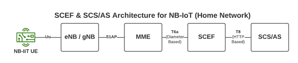
To support this we introduce a new network element called the SCEF –Service Capability Exposure Function.
From a developer’s perspective, the SCEF is the gateway to our IoT devices. Through the RESTful API on the SCEF (T8 API), we can send and receive raw hex data to any of our IoT devices.
When one of our Water-as-a-Service Taps sends usage data as a hex byte, it’s the software talking on the T8 API to the SCEF that receives this data.
Data of course needs to be addressed, so we know where it’s coming from / going to, and T8 handles this, as well as message reliability, etc, etc.
This is a telco blog, so we should probably cover the MME connection, the MME talks via Diameter to the SCEF. In our next post we’ll go into these signaling flows in more detail.
If you’re wondering what the status of Open Source SCEF implementations are, then you may have already guessed I’m working on one!
Hopefully by now you’ve got a bit of an idea of how NIDD works in NB-IoT, and in our next posts we’ll dig deeper into the flows and look at some PCAPs together.
Having a central pair of Diameter routing agents allows us to drastically simplify our network, but what if we want to perform some translations on AVPs?
For starters, what is an AVP transformation? Well it’s simply rewriting the value of an AVP as the Diameter Request/Response passes through the DRA. A request may come into the DRA with IMSI xxxxxx and leave with IMSI yyyyyy if a translation is applied.
So why would we want to do this?
Well, what if we purchased another operator who used Realm X, and we use Realm Y, and we want to link the two networks, then we’d need to rewrite Realm Y to Realm X, and Realm X to Realm Y when they communicate, AVP transformations allow for this.
If we’re an MVNO with hosted IMSIs from an MNO, but want to keep just the one IMSI in our HSS/OCS, we can translate from the MNO hosted IMSI to our internal IMSI, using AVP transformations.
If our OCS supports only one rating group, and we want to rewrite all rating groups to that one value, AVP transformations cover this too.
There are lots of uses for this, and if you’ve worked with a bit of signaling before you’ll know that quite often these sorts of use-cases come up.
So how do we do this with freeDiameter?
To handle this I developed a module for passing each AVP to a Python function, which can then apply any transformation to a text based value, using every tool available to you in Python.
In the next post I’ll introduce rt_pyform and how we can use it with Python to translate Diameter AVPs.
What I typically refer to as Diameter interfaces / reference points, such as S6a, Sh, Sx, Sy, Gx, Gy, Zh, etc, etc, are also known as Applications.
Diameter Application Support
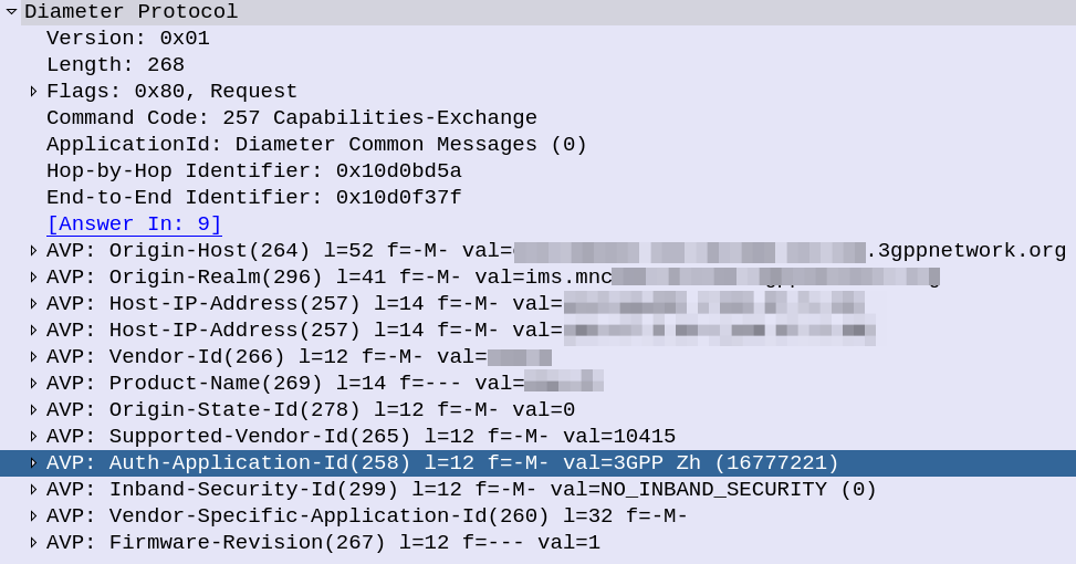
If you look inside the Capabilities Exchange Request / Answer dialog, what you’ll see is each side advertising the Applications (interfaces) that they support, each one being identified by an Application ID.
CER showing support for the 3GPP Zh Application-ID (Interface)
If two peers share a common Application-Id, then they can communicate using that Application / Interface.
For example, the above screenshot shows a peer with support for the Zh Interface (Spoiler alert, XCAP Gateway / BSF coming soon!). If two Diameter peers both have support for the Zh interface, then they can use that to send requests / responses to each other.
This is the basis of Diameter Routing.
Diameter Routing Tables
Like any router, our DRA needs to have logic to select which peer to route each message to.
For each Diameter connection to our DRA, it will build up a Diameter Routing table, with information on each peer, including the realm and applications it advertises support for.
Then, based on the logic defined in the DRA to select which Diameter peer to route each request to.
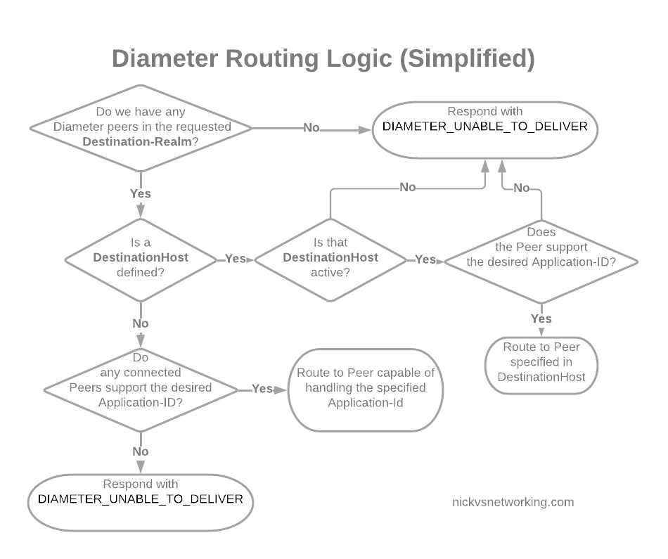
In its simplest form, Diameter routing is based on a few things:
Look at the DestinationRealm, and see if we have any peers at that realm
If we do then look at the DestinationHost, if that’s set, and the host is connected, and if it supports the specified Application-Id, then route it to that host
If no DestinationHost is specified, look at the peers we have available and find the one that supports the specified Application-Id, then route it to that host
Simplified Diameter Routing Table used by DRAs
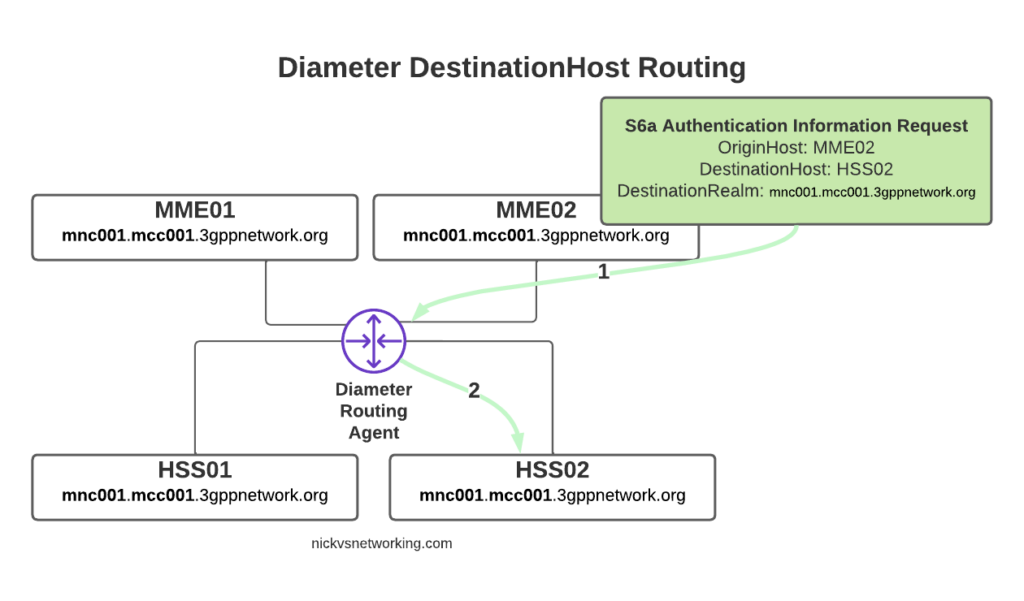
With this in mind, we can go back to looking at how our DRA may route a request from a connected MME towards an HSS.
Let’s look at some examples of this at play.
The request from MME02 is for DestinationRealm mnc001.mcc001.3gppnetwork.org, which our DRA knows it has 4 connected peers in (3 if we exclude the source of the request, as we don’t want to route it back to itself of course).
So we have 3 contenders still for who could get the request, but wait! We have a DestinationHost specified, so the DRA confirms the host is available, and that it supports the requested ApplicationId and routes it to HSS02.
So just because we are going through a DRA does not mean we can’t specific which destination host we need, just like we would if we had a direct link between each Diameter peer.
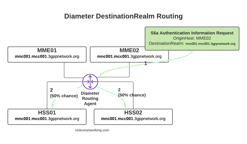
Conversely, if we sent another S6a request from MME01 but with no DestinationHost set, let’s see how that would look.
Again, the request is from MME02 is for DestinationRealm mnc001.mcc001.3gppnetwork.org, which our DRA knows it has 3 other peers it could route this to. But only two of those peers support the S6a Application, so the request would be split between the two peers evenly.
Clever Routing with DRAs
So with our DRA in place we can simplify the network, we don’t need to build peer links between every Diameter device to every other, but let’s look at some other ways DRAs can help us.
Load Control
We may want to always send requests to HSS01 and only use HSS02 if HSS01 is not available, we can do this with a DRA.
Or we may want to split load 75% on one HSS and 25% on the other.
Both are great use cases for a DRA.
Routing based on Username
We may want to route requests in the DRA based on other factors, such as the IMSI.
Our IMSIs may start with 001010001xxx, but if we introduced an MVNO with IMSIs starting with 001010002xxx, we’d need to know to route all traffic where the IMSI belongs to the home network to the home network HSS, and all the MVNO IMSI traffic to the MVNO’s HSS, and DRAs handle this.
Inter-Realm Routing
One of the main use cases you’ll see for DRAs is in Roaming scenarios.
For example, if we have a roaming agreement with a subscriber who’s IMSIs start with 90170, we can route all the traffic for their subs towards their HSS.
But wait, their Realm will be mnc901.mcc070.3gppnetwork.org, so in that scenario we’ll need to add a rule to route the request to a different realm.
DRAs handle this also.
In our next post we’ll start actually setting up a DRA with a default route table, and then look at some more advanced options for Diameter routing like we’ve just discussed.
One slight caveat, is that mutual support does not always mean what you may expect. For example an MME and an HSS both support S6a, which is identified by Auth-Application-Id 16777251 (Vendor ID 10415), but one is a client and one is a server. Keep this in mind!
Answer Question 1: Because they make things simpler and more flexible for your Diameter traffic. Answer Question 2: With free software of course!
All about DRAs
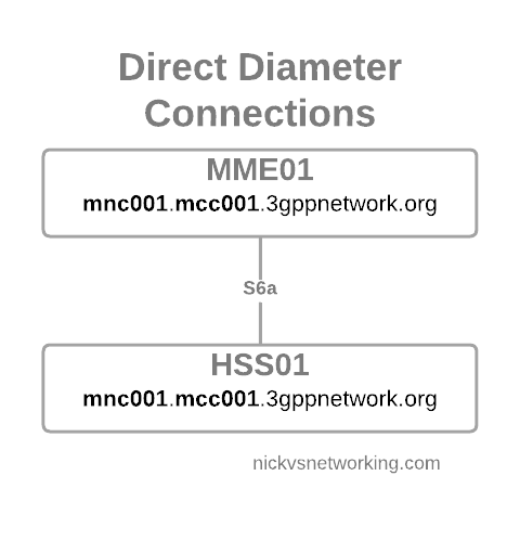
But let’s dive a little deeper. Let’s look at the connection between an MME and an HSS (the S6a interface).
Direct Diameter link between two Diameter Peers
We configure the Diameter peers on MME1 and HSS01 so they know about each other and how to communicate, the link comes up and presto, away we go.
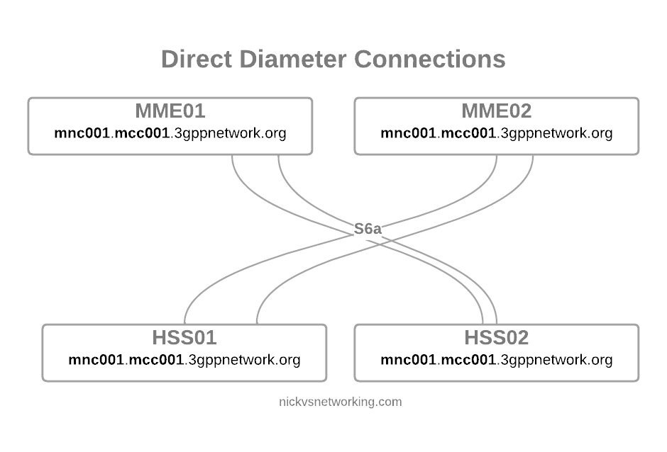
But we’re building networks here! N+1 redundancy and all that, so now we have two HSSes and two MMEs.
Direct Diameter link between 4 Diameter peers
Okay, bit messy, but that’s okay…
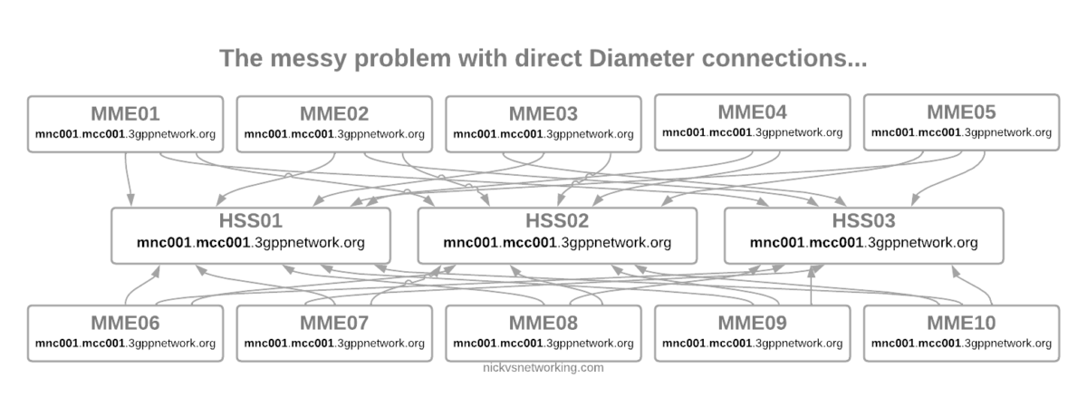
But then our network grows to 10 MMEs, and 3 HSSes and you can probably see where this is going, but let’s drive the point home.
Direct Diameter connections for a network with 10x MME and 3x HSS
Now imagine once you’ve set all this up you need to do some maintenance work on HSS03, so need to shut down the Diameter peer on 10 different MMEs in order to isolate it and deisolate it.
The problem here is pretty evident, all those links are messy, cumbersome and they just don’t scale.
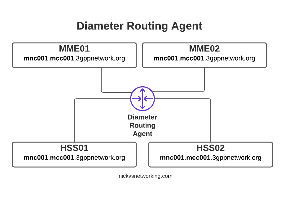
If you’re someone with a bit of networking experience (and let’s face it, you’re here after all), then you’re probably thinking “What if we just had a central system to route all the Diameter messages?”
An Agent that could Route Diameter, a Diameter Routing Agent perhaps…
By introducing a DRA we build Diameter peer links between each of our Diameter devices (MME / HSS, etc) and the DRA, rather than directly between each peer.
With Diameter Routing Agent
Then from the DRA we can route Diameter requests and responses between them.
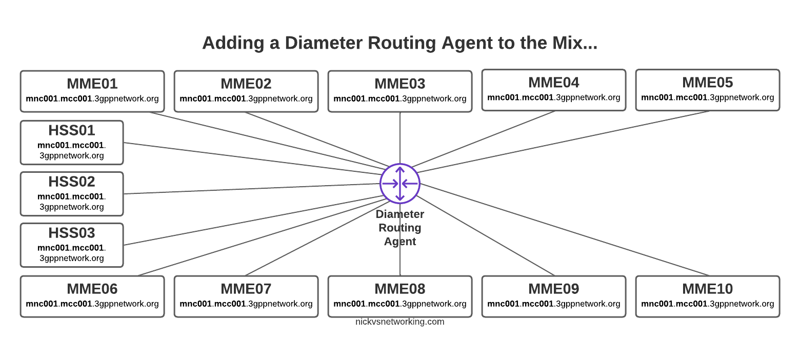
Let’s go back to our 10x MME and 3x HSS network and see how it looks with a DRA instead.
So much cleaner!
Not only does this look better, but it makes our life operating the network a whole lot easier.
Each MME sends their S6a traffic to the DRA, which finds a healthy HSS from the 3 and sends the requests to it, and relays the responses as well.
We can do clever load balancing now as well.
Plus if a peer goes down, the DRA detects the failure and just routes to one of the others.
If we were to introduce a new HSS, we wouldn’t need to configure anything on the MMEs, just add HSS04 to the DRA and it’ll start getting traffic.
Plus from an operations standpoint, now if we want to to take an HSS offline for maintenance, we just shut down the link on the HSS and all HSS traffic will get routed to the other two HSS instances.
In our next post we’ll talk about the Routing part of the DRA, how the decisions are made and all the nuances, and then in the following post we’ll actually build a DRA and start routing some traffic around!
Carl Sagan once famously said “If you wish to make an apple pie from scratch, you must first invent the universe”, we don’t need to go that far back, but if you want to deliver an MMS to a subscriber, first you must deliver an SMS.
Wait, but we’re talking about MMS right? So why are we talking SMS?
Modern MMS transport relies on HTTP, which is client-server based, the phone / UE is the client, and the MMSc is the Server.
The problem with this client-server relationship, is the client requests things from the server, but the server can’t request things from the client.
This presents a problem when it comes to delivering the MMS – The phone / UE will need to request the MMSc provide it the message to be received, but needs to know there is a message to request in the first place.
So this is where SMS comes in. When the MMSc has a message destined for a Subscriber, it sends the phone/UE an SMS, informing that there is an MMS waiting, and providing the URL the MMS can be retrieved from.
This is typically done by MAP or SMPP, to link the MMSc to the SMSc to allow it to send these messages.
This SMS contains the URL to retrieve the MMS at, once the UE receives this SMS, it knows where to retrieve the MMS.
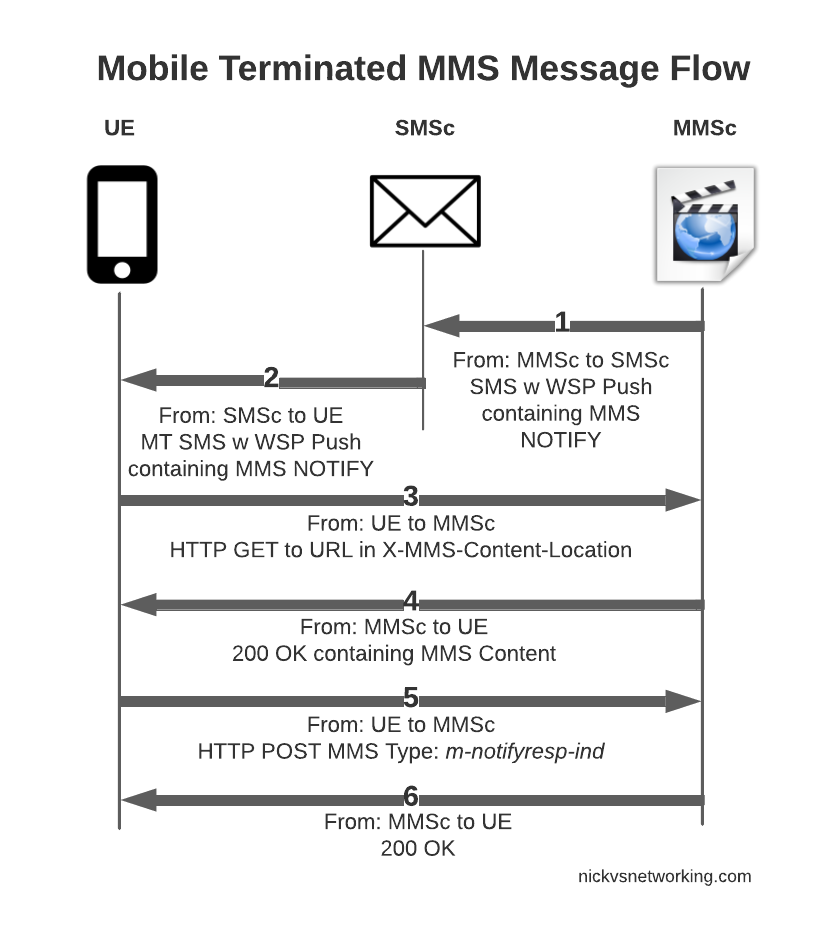
It can then send an HTTP GET to the URL to retrieve the MMS, and lastly sends an HTTP POST to confirm to the MMSc it retrieved it all OK.
MMS Mobile Terminated message flow
So that’s the basics, let’s look at each part of the dialog in some more detail, starting with this magic SMS to tell the UE where to retrieve the MMS from.
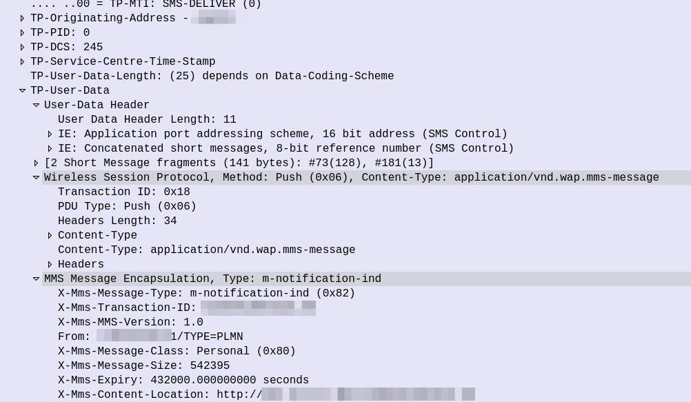
WAP PUSH from MMSc sent via SMS
So some things to notice, the user data, which would usually carry the body of our SMS instead contains another protocol, “Wireless Session Protocol” (WSP), and this is the method “Push”.
That in turn is followed by MMS Message Encapsulation, again inside the SMS message body, this time with the MMS specific data.
The From: header contains the sender of the MMS, this is how you can see who the MMS is from, while it’s still downloading.
The expiry indicates to the handset, it it doesn’t download the MMS within the specified time period, it shouldn’t bother, as the message will have expired.
And lastly, and perhaps most importantly, we have the X-MMS-Content-Location header, which tells our subscriber where to download the MMS from.
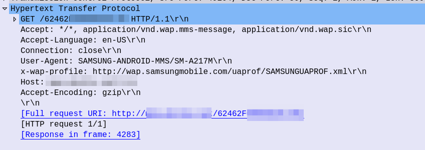
After this, the UE sends an HTTP GET to the URL in the X-MMS-Content-Location header (typically on the “mms” APN), to retrieve the MMS from the MMSc.
HTTP GET from the UE to the MMSc
The HTTP GET is pretty normal, there’s the usual MMS headers we talked about in the last post, and we just GET the path provided by the MMSc in the WAP PUSH.
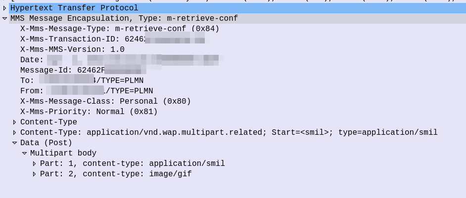
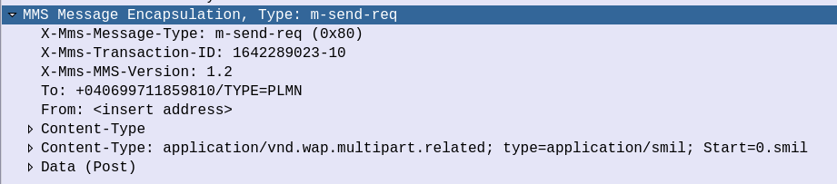
The response from the MMSc contains the actual MMS itself, which is almost a mirror of the sending process (the Data component is unchanged from when the sender sent it).
Response to HTTP GET for message retrieval
At this stage our subscriber has retrieve the MMS, but may not have retrieved it fully, or may have had an issue retrieving it.
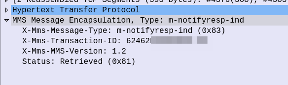
Instead the UE sends an HTTP POST with the MMS-Message-Type m-notifyresp-ind with the transaction ID, to indicate that it has successfully retrieved the MMS, and at this point the MMS can notify the sender if delivery receipts are enabled, and delete the message from the cache.
And finally the MMSc sends back a 200 OK with no body to confirm it got that too.
Some notes on MMS Security
Reading about unauthenticated GET requests, you may be left wondering what security does MMS have, and what stops you from just going through and sending HTTP GET requests to all the possible URL paths to vacuum up all the MMS?
In the standard, nothing!
Typically the MMSc has some layer of security added by the implementer, to ensure the user retrieving the MMS, is the user the MMS is destined for. Because MMS has no security in the standard, this is typically achieved through Header Enrichment, whereby the P-GW adds a HTTP header with the MSISDN or IMSI of the subscriber, and then the MMSc can evaluate if this subscriber should be able to retrieve that URL.
Another attack vector I played with was sending a SMS based MMS-Notify with a different URL, which if retrieved, would leak the subscriber’s IP, as it would cause the UE to try and get data from that URL.
Recently I had a strange issue I thought I’d share.
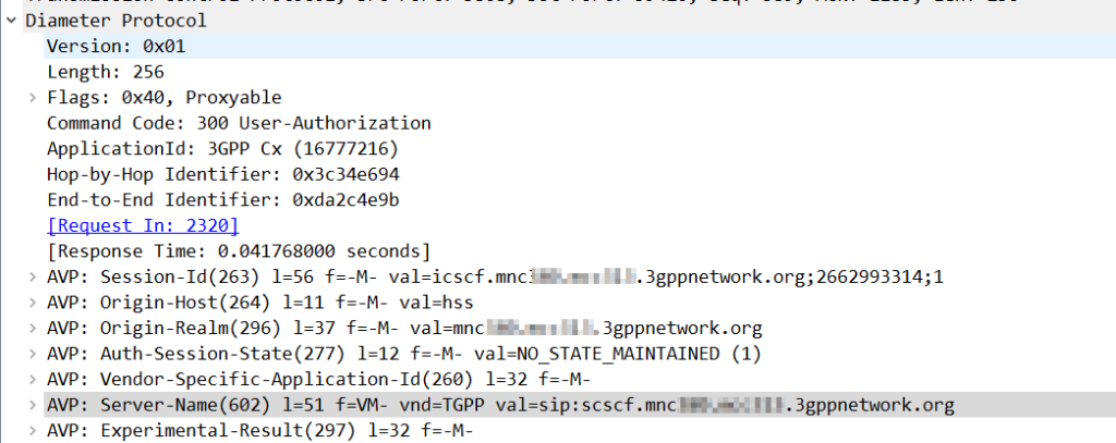
Using Kamailio as an Interrogating-CSCF, Kamailio was getting the S-CSCF details from the User-Authorization-Answer’s “Server-Name” (602) AVP.
The value was set to:
sip:scscf.mnc001.mcc001.3gppnetwork.org:5060
But the I-CSCF was only looking up A-Records for scscf.mnc001.mcc001.3gppnetwork.org, not using DNS-SRV.
The problem? The Server-Name I had configured as a full SIP URI in PyHSS including the port, meant that Kamailio only looks up the A-Record, and did not do a DNS-SRV lookup for the domain.
Dropping the port number saw all those delicious SRV records being queried.
Something to keep in mind if you use S-CSCF pooling with a Kamailio based I-CSCF, if you want to use SRV records for load balancing / traffic sharing, don’t include the port, and if instead you want it to go to the specified host found by an A-record, include the port.
So you want to send a Multimedia Message (Aka MMS or MM)?
Let’s do it – We’ll use the MM1 interface from the UE towards the MMSc (MMS Service Center) to send our Mobile Originated MMS.
Transport & Creation
Out of the box, our UE doesn’t get told by the network anything about where to send MMS messages (Unless set via something like Android’s Carrier Settings). Instead, this is typically configured by the user in the APN settings, by setting the MMSc address (Typically an FQDN), port (Typically 80) and often a Proxy (Which will actually handle the traffic). Lastly under the bearer type, if we’re sending the MMS on the default bearer (the one used for general Internet) then the bearer type will need to change from “default” to “default,mms”. Alternately, if you’re using a dedicated APN for MMS, you’ll need to set the bearer type to “mms”.
With the connectivity side setup, we’ll need to actually generate an MMS to send, something that is encapsulated in an MMS – so a picture is a good start.
We compose a message with this photo, put an address in the message and hit send on the UE.
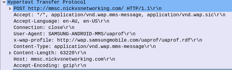
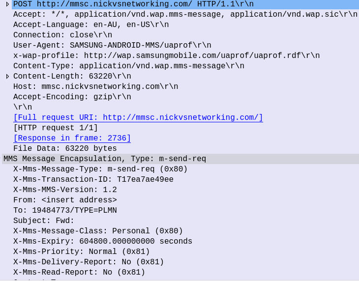
The UE encapsulates the photo and metadata, such as the To address, into an HTTP POST is sent to the IP & Port of your MMSc (Or proxy if you have that set). The body of this HTTP POST contains the MMS Message Body (In this case our picture).
Our MMSc receives this POST, extracts the headers of interest, and the multimedia message body itself (in our case the photo) ready to be forwarded onto their destination.
PCAP Extract showing MMS m-send-req from UE
Header Enrichment / Charging / Authentication
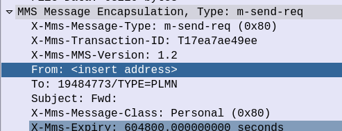
One thing to note is that the From header is empty.
Often times a UE doesn’t know it’s own MSISDN. While there is an MSISDN EF on the SIM file system, often this is not updated with the correct MSISDN, as a customer may have ported over their number from a different carrier, or had a replacement SIM reissued. There’s also some problems in just trusting the From address set by a UE, without verifying it as anyone could change this.
The MMS standards evolved in parallel to the 3GPP specifications, but were historically specified by the Open Mobile Alliance. Because it is at arms length with 3GPP, SIM based authentication was not used on the MM1 interface from a UE to the MMSc.
In fact, there is no authentication on an MMS specified in the standard, meaning in theory, anyone could send one. To counter this, the P-GW or GGSN handling the subscriber traffic often enables “Header Enrichment” which when it detects traffic on the MMS APN, will add a Header to the Mobile Originated request with the IMSI or MSISDN of the subscriber sending it, which the MMSc can use to bill the customer.
m-send-req Request
Let’s take a closer look into the HTTP POST sent by the UE containing the message.
Firstly we have what looks like a pretty bulk-standard HTTP POST header, albeit with some custom headers prefixed with “X-” and the Content-Type is application/vnd.wap.mms-message.
But immediately after the HTTP header in the HTTP message body, we have the “MMS Message Encapsulation” header:
MMS Message Encapsulation Header from MO MMS
This header contains the Destination we set in the MMS when sending it, the request type (m-send-req) as well as the actual content itself (inside the Data section).
So why the double header? Why not just encapsulate the whole thing in the HTTP Post? When MMS was introduced, most phones didn’t have a HTTP stack baked into them like everything does now. Instead traffic would be going through a WAP Gateway.
When usage of WAP fell away, the standard moved to transport the same payload that was transfered over WAP, to instead be transferred over HTTP.
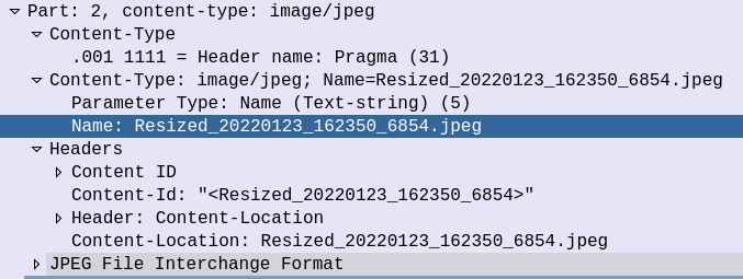
Inside the Data section we can see the MIME Type of the attachments themselves, in this case, it’s a photo of my desk:
With all this information, the MMSc analyses the headers and stores the message body ready for forwarding onto the recipient(/s).
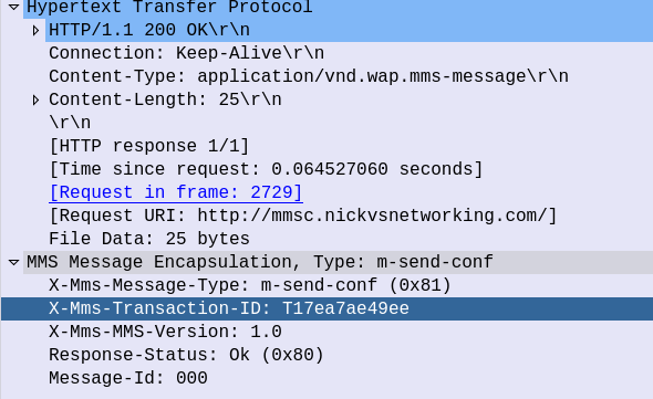
m-send-conf Response
To confirm successful receipt, the MMSc sends back a 200 OK with a matching Transaction ID, so the UE knows the message was accepted.
I’ve recently been writing a lot about SS7 / Sigtran, and couldn’t fit this in anywhere, but figured it may be of use to someone…
In our 3-8-3 formated ITU International Point code, each of the parts have a unique meaning.
The 3 bits in the first section are called the Zone section. Being only 3 bits long it means we can only encode the numbers 0-7 on them, but ITU have broken the planet up into different “zones”, so the first part of our ITU International Point Code denotes which Zone the Point Code is in (as allocated by ITU).
The next 8 bits in the second section (Area section) are used to define the “Signaling Area Network Code” (SANC), which denotes which country a point code is located in. Values can range from 0-255 and many countries span multiple SANC zones, for example the USA has 58 SANC Zones.
Lastly we have the last 3 bits that make up the ID section, denoting a single unique point code, typically a carrier’s international gateway. It’s unique within a Zone & SANC, so combined with the Zone-SANC-ID makes it a unique address on the SS7 network. Being only 3 bits long means that we’ve only got 8 possible values, hence so many SANCs being used.
2
Europe
3
Greenland, North America, the Caribbean, and Mexico
This is part of a series of posts looking into SS7 and Sigtran networks. We cover some basic theory and then get into the weeds with GNS3 based labs where we will build real SS7/Sigtran based networks and use them to carry traffic.
Having a direct Linkset from every Point Code to every other Point Code in an SS7 network isn’t practical, we need to rely on routing, so in this post we’ll cover routing between Point Codes on our STPs.
Let’s start in the IP world, imagine a router with a routing table that looks something like this:
Simple IP Routing Table
192.168.0.0/24 out 192.168.0.1 (Directly Attached)
172.16.8.0/22 via 192.168.0.3 - Static Route - (Priority 100)
172.16.0.0/16 via 192.168.0.2 - Static Route - (Priority 50)
10.98.22.1/32 via 192.168.0.3 - Static Route - (Priority 50)
We have an implicit route for the network we’re directly attached to (192.168.0.0/24), and then a series of static routes we configure. We’ve also got two routes to the 172.16.8.0/22 subnet, one is more specific with a higher priority (172.16.8.0/22 – Priority 100), while the other is less specific with a lower priority (172.16.0.0/16 – Priority 50). The higher priority route will take precedence.
This should look pretty familiar to you, but now we’re going to take a look at routing in SS7, and for that we’re going to be talking Variable Length Subnet Masking in detail you haven’t needed to think about since doing your CCNA years ago…
Why Masking is Important
A route to a single Point Code is called a “/14”, this is akin to a single IPv4 address being called a “/32”.
We could setup all our routing tables with static routes to each point code (/14), but with about 4,000 international point codes, this might be a challenge.
Instead, by using Masks, we can group together ranges of Point Codes and route those ranges through a particular STP.
This opens up the ability to achieve things like “Route all traffic to Point Codes to this Default Gateway STP”, or to say “Route all traffic to this region through this STP”.
Individually routing to a point code works well for small scale networking, but there’s power, flexibility and simplification that comes from grouping together ranges of point codes.
Information Overload about Point Codes
So far we’ve talked about point codes in the X.YYY.Z format, in our lab we setup point codes like 1.2.3.
This is not the only option however…
Variants of SS7 Point Codes
IPv4 addresses look the same regardless of where you are. From Algeria to Zimbabwe, IPv4 addresses look the same and route the same.
In SS7 networks that’s not the case – There are a lot of variants that define how a point code is structured, how long it is, etc. Common variants are ANSI, ITU-T (International & National variants), ETSI, Japan NTT, TTC & China.
The SS7 variant used must match on both ends of a link; this means an SS7 node speaking ETSI flavoured Point Codes can’t exchange messages with an ANSI flavoured Point Code.
Well, you can kinda translate from one variant to another, but requires some rewriting not unlike how NAT does it.
ITU International Variant
For the start of this series, we’ll be working with the ITU International variant / flavour of Point Code.
ITU International point codes are 14 bits long, and format is described as 3-8-3. The 3-8-3 form of Point code just means the 14 bit long point code is broken up into three sections, the first section is made up of the first 3 bits, the second section is made up of the next 8 bits then the remaining 3 bits in the last section, for a total of 14 bits.
So our 14 bit 3-8-3 Point Code looks like this in binary form:
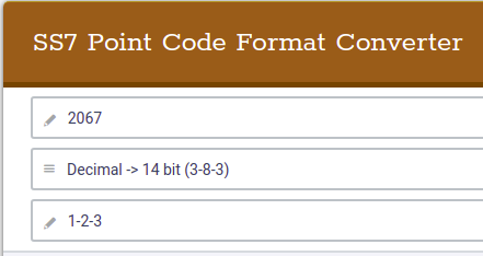
If you’re dealing with multiple vendors or products,you’ll see some SS7 Point Codes represented as decimal (2067), some showing as 1-2-3 codes and sometimes just raw binary. Fun hey?
So why does the binary part matter? Well the answer is for masks.
To loop back to the start of this post, we talked about IP routing using a network address and netmask, to represent a range of IP addresses. We can do the same for SS7 Point Codes, but that requires a teeny bit of working out.
As an example let’s imagine we need to setup a route to all point codes from 3-4-0 through to 3-6-7, without specifying all the individual point codes between them.
Firstly let’s look at our start and end point codes in binary:
100-00000100-000 = 3-004-0 (Start Point Code)
100-00000110-111 = 3-006-7 (End Point Code)
Looking at the above example let’s look at how many bits are common between the two,
100-00000100-000 = 3-004-0 (Start Point Code)
100-00000110-111 = 3-006-7 (End Point Code)
The first 9 bits are common, it’s only the last 5 bits that change, so we can group all these together by saying we have a /9 mask.
When it comes time to add a route, we can add a route to 3-4-0/9 and that tells our STP to match everything from point code 3-4-0 through to point code 3-6-7.
The STP doing the routing it only needs to match on the first 9 bits in the point code, to match this route.
SS7 Routing Tables
Now we have covered Masking for roues, we can start putting some routes into our network.
In order to get a message from one point code to another point code, where there isn’t a direct linkset between the two, we need to rely on routing, which is performed by our STPs.
This is where all that point code mask stuff we just covered comes in.
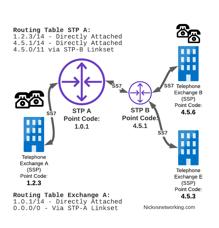
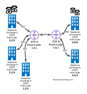
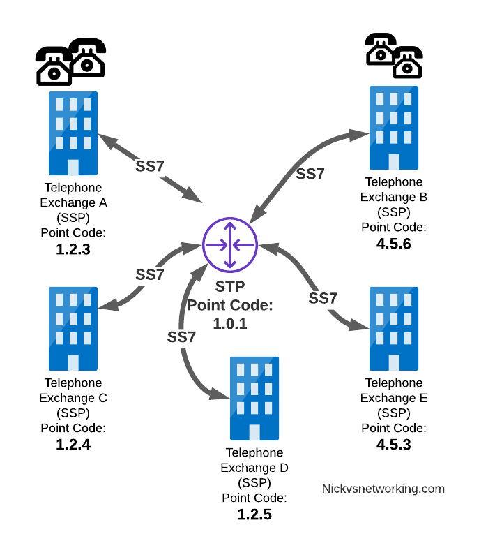
Let’s look at a diagram below,
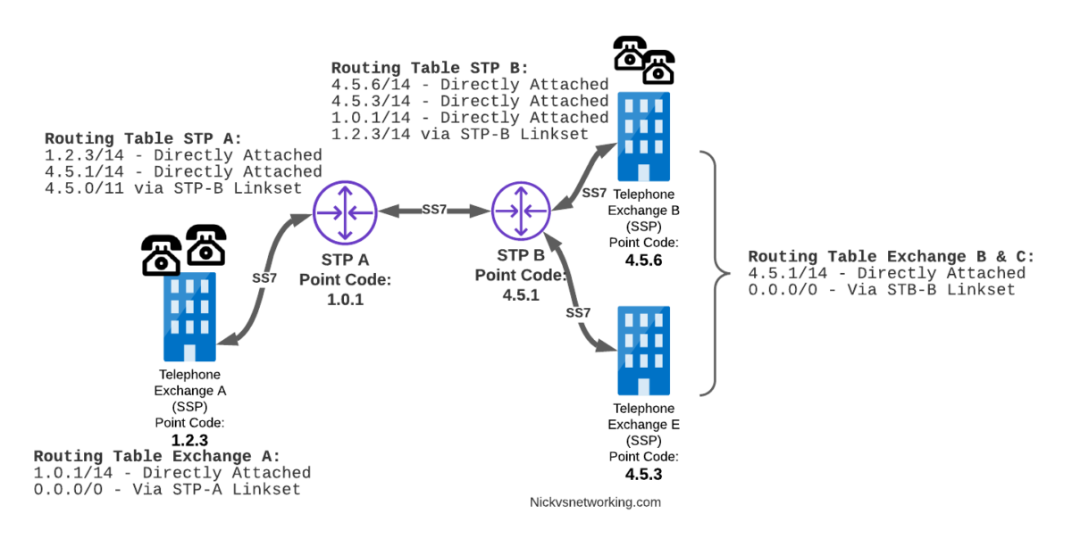
Let’s look at the routing to get a message from Exchange A (SSP) on the bottom left of the picture to Exchange E (SSP) with Point Code 4.5.3 in the bottom right of the picture.
Exchange A (SSP) on the bottom left of the picture has point code 1.2.3 assigned to it and a Linkset to STP-A. It has the implicit route to STP-A as it’s got that linkset, but it’s also got a route configured on it to reach any other point code via the Linkset to STP-A via the 0.0.0/0 route which is the SS7 equivalent of a default route. This means any traffic to any point code will go to STP-A.
From STP-A we have a linkset to STP-B. In order to route to the point codes behind STP-B, STP-A has a route to match any Point Code starting with 4.5.X, which is 4.5.0/11. This means that STP-A will route any Point Code between 4.5.1 and 4.5.7 down the Linkset to STP-B.
STP-B has got a direct connection to Exchange B and Exchange E, so has implicit routes to reach each of them.
So with that routing table, Exchange A should be able to route a message to Exchange E.
But…
Return Routing
Just like in IP routing, we need return routing. while Exchange A (SSP) at 1.2.3 has a route to everywhere in the network, the other parts of the network don’t have a route to get to it. This means a request from 1.2.3 can get anywhere in the network, but it can’t get a response back to 1.2.3.
So to get traffic back to Exchange A (SSP) at 1.2.3, our two Exchanges on the right (Exchange B & C with point codes 4.5.6 and 4.5.3) will need routes added to them. We’ll also need to add routes to STP-B, and once we’ve done that, we should be able to get from Exchange A to any point code in this network.
There is a route missing here, see if you can pick up what it is!
So we’ve added a default route via STP-B on Exchange B & Exchange E, and added a route on STP-B to send anything to 1.2.3/14 via STP-A, and with that we should be able to route from any exchange to any other exchange.
One last point on terminology – when we specify a route we don’t talk in terms of the next hop Point Code, but the Linkset to route it down. For example the default route on Exchange A is 0.0.0/0 via STP-A linkset (The linkset from Exchange A to STP-A), we don’t specify the point code of STP-A, but just the name of the Linkset between them.
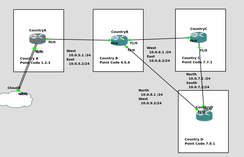
Back into the Lab
So back to the lab, where we left it was with linksets between each point code, so each Country could talk to it’s neighbor.
Let’s confirm this is the case before we go setting up routes, then together, we’ll get a route from Country A to Country C (and back).
So let’s check the status of the link from Country B to its two neighbors – Country A and Country C. All going well it should look like this, and if it doesn’t, then stop by my last post and check you’ve got everything setup.
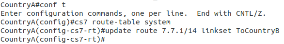
So let’s add some routing so Country A can reach Country C via Country B. On Country A STP we’ll need to add a static route. For this example we’ll add a route to 7.7.1/14 (Just Country C).
That means Country A knows how to get to Country C. But with no return routing, Country C doesn’t know how to get to Country A. So let’s fix that.
We’ll add a static route to Country C to send everything via Country B.
CountryC#conf t
Enter configuration commands, one per line.  End with CNTL/Z.
CountryC(config)#cs7 route-table system
CountryC(config)#update route 0.0.0/0 linkset ToCountryB
*Jan 01 05:37:28.879: %CS7MTP3-5-DESTSTATUS: Destination 0.0.0 is accessible
So now from Country C, let’s see if we can ping Country A (Ok, it’s not a “real” ICMP ping, it’s a link state check message, but the result is essentially the same).
By running:
CountryC# ping cs7 1.2.3
*Jan 01 06:28:53.699: %CS7PING-6-RTT: Test Q.755 1.2.3: MTP Traffic test rtt 48/48/48
*Jan 01 06:28:53.699: %CS7PING-6-STAT: Test Q.755 1.2.3: MTP Traffic test 100% successful packets(1/1)
*Jan 01 06:28:53.699: %CS7PING-6-RATES: Test Q.755 1.2.3: Receive rate(pps:kbps) 1:0 Sent rate(pps:kbps) 1:0
*Jan 01 06:28:53.699: %CS7PING-6-TERM: Test Q.755 1.2.3: MTP Traffic test terminated.
We can confirm now that Country C can reach Country A, we can do the same from Country A to confirm we can reach Country B.
But what about Country D? The route we added on Country A won’t cover Country D, and to get to Country D, again we go through Country B.
This means we could group Country C and Country D into one route entry on Country A that matches anything starting with 7-X-X,
For this we’d add a route on Country A, and then remove the original route;
Of course, you may have already picked up, we’ll need to add a return route to Country D, so that it has a default route pointing all traffic to STP-B. Once we’ve done that from Country A we should be able to reach all the other countries:
CountryA#show cs7 route
Dynamic Routes 0 of 1000

Routing table = system Destinations = 3 Routes = 3

Destination            Prio Linkset Name        Route
---------------------- ---- ------------------- -------
4.5.6/14         acces   1  ToCountryB          avail
7.0.0/3          acces   5  ToCountryB          avail


CountryA#ping cs7 7.8.1
*Jan 01 07:28:19.503: %CS7PING-6-RTT: Test Q.755 7.8.1: MTP Traffic test rtt 84/84/84
*Jan 01 07:28:19.503: %CS7PING-6-STAT: Test Q.755 7.8.1: MTP Traffic test 100% successful packets(1/1)
*Jan 01 07:28:19.503: %CS7PING-6-RATES: Test Q.755 7.8.1: Receive rate(pps:kbps) 1:0  Sent rate(pps:kbps) 1:0
*Jan 01 07:28:19.507: %CS7PING-6-TERM: Test Q.755 7.8.1: MTP Traffic test terminated.
CountryA#ping cs7 7.7.1
*Jan 01 07:28:26.839: %CS7PING-6-RTT: Test Q.755 7.7.1: MTP Traffic test rtt 60/60/60
*Jan 01 07:28:26.839: %CS7PING-6-STAT: Test Q.755 7.7.1: MTP Traffic test 100% successful packets(1/1)
*Jan 01 07:28:26.839: %CS7PING-6-RATES: Test Q.755 7.7.1: Receive rate(pps:kbps) 1:0  Sent rate(pps:kbps) 1:0
*Jan 01 07:28:26.843: %CS7PING-6-TERM: Test Q.755 7.7.1: MTP Traffic test terminated.
So where to from here?
Well, we now have a a functional SS7 network made up of STPs, with routing between them, but if we go back to our SS7 network overview diagram from before, you’ll notice there’s something missing from our lab network…
So far our network is made up only of STPs, that’s like building a network only out of routers!
In our next lab, we’ll start adding some SSPs to actually generate some SS7 traffic on the network, rather than just OAM traffic.
This is part of a series of posts looking into SS7 and Sigtran networks. We cover some basic theory and then get into the weeds with GNS3 based labs where we will build real SS7/Sigtran based networks and use them to carry traffic.
So we’ve made it through the first two parts of this series talking about how it all works, but now dear reader, we build an SS7 Lab!
At one point, and SS7 Signaling Transfer Point would be made up of at least 3 full size racks, and cost $5M USD. We can run a dozen of them inside GNS3!
Cisco’s “IP Transfer Point” (ITP) software adds SS7 STP functionality to some models of Cisco Router, like the 2651XM and C7200 series hardware.
Luckily for us, these hardware platforms can be emulated in GNS3, so that’s how we’ll be setting up our instances of Cisco’s ITP product to use as STPs in our network.
For the rest of this post series, I’ll refer to Cisco’s IP Transfer Point as the “Cisco STP”.
Not open source you say! Osmocom have OsmoSTP, which we’ll introduce in a future post, and elaborate on why later…
From inside GNS3, we’ll create a new template as per the Gif below.
You will need a copy of the software image to load in. If you’ve got software entitlements you should be able to download it, the filename of the image I’m using for the 7200 series is c7200-itpk9-mz.124-15.SW.bin and if you go searching, you should find it.
Now we can start building networks with our Cisco STPs!
What we’re going to achieve
In this lab we’re going to introduce the basics of setting up STPs using Sigtran (SS7 over IP).
If you follow along, by the end of this post you should have two STPs talking Sigtran based SS7 to each other, and be able to see the SS7 packets in Wireshark.
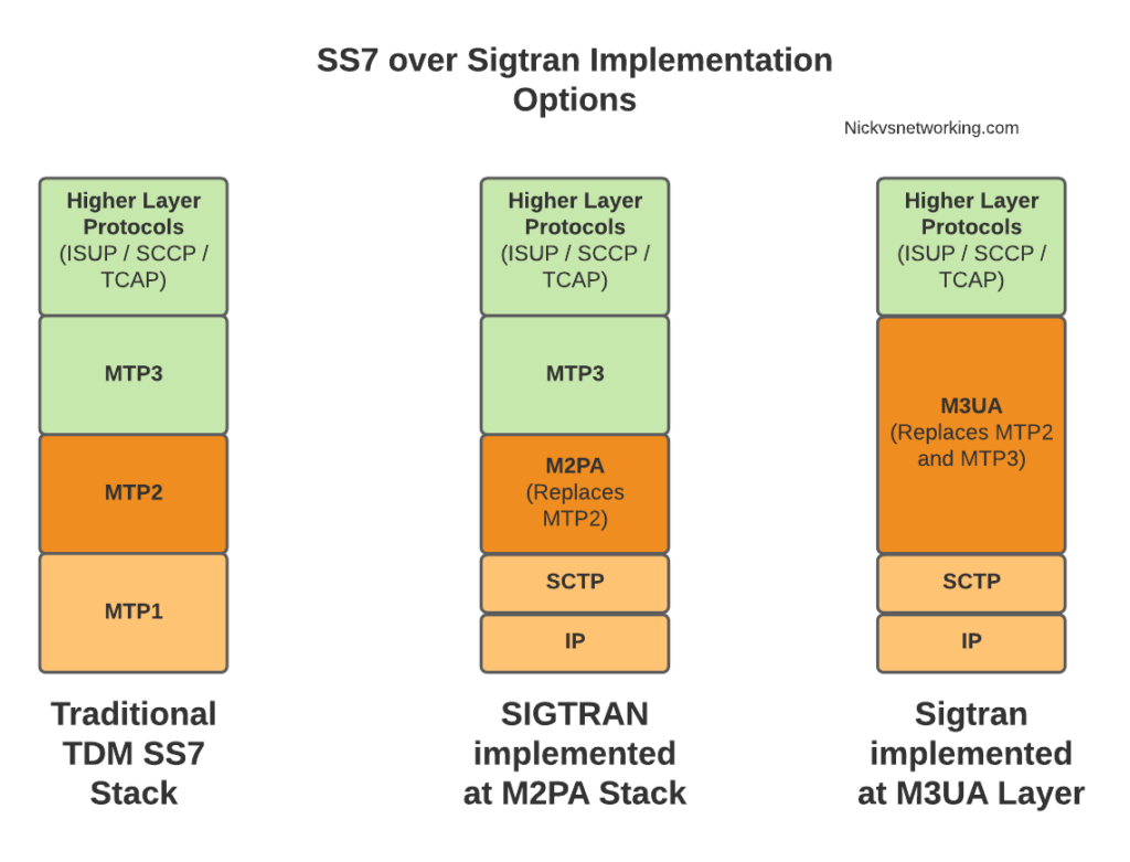
As we touched on in the last post, there’s a lot of different flavours and ways to implement SS7 over IP. For this post, we’re going to use M2PA (MTP2 Peer Adaptation Layer) to carry the MTP2 signaling, while MTP3 and higher will look the same as if it were on a TDM link. In a future post we’ll better detail the options here, the strengths and weaknesses of each method of transporting SS7 over IP, but that’s future us’ problem.
IP Connectivity
As we don’t have any TDM links, we’re going to do everything on IP, this means we have to setup the IP layer, before we can add any SS7/Sigtran stuff on top, so we’re going to need to get basic IP connectivity going between our Cisco STPs.
So for this we’ll need to set an IP Address on an interface, unshut it, link the two STPs. Once we’ve confirmed that we’ve got IP connectivity running between the two, we can get started on the Sigtran / SS7 side of things.
Let’s face it, if you’re reading this, I’m going to bet that you are probably aware of how to configure a router interface.
I’ve put a simple template down in the background to make a little more sense, which I’ve attached here if you want to follow along with the same addressing, etc.
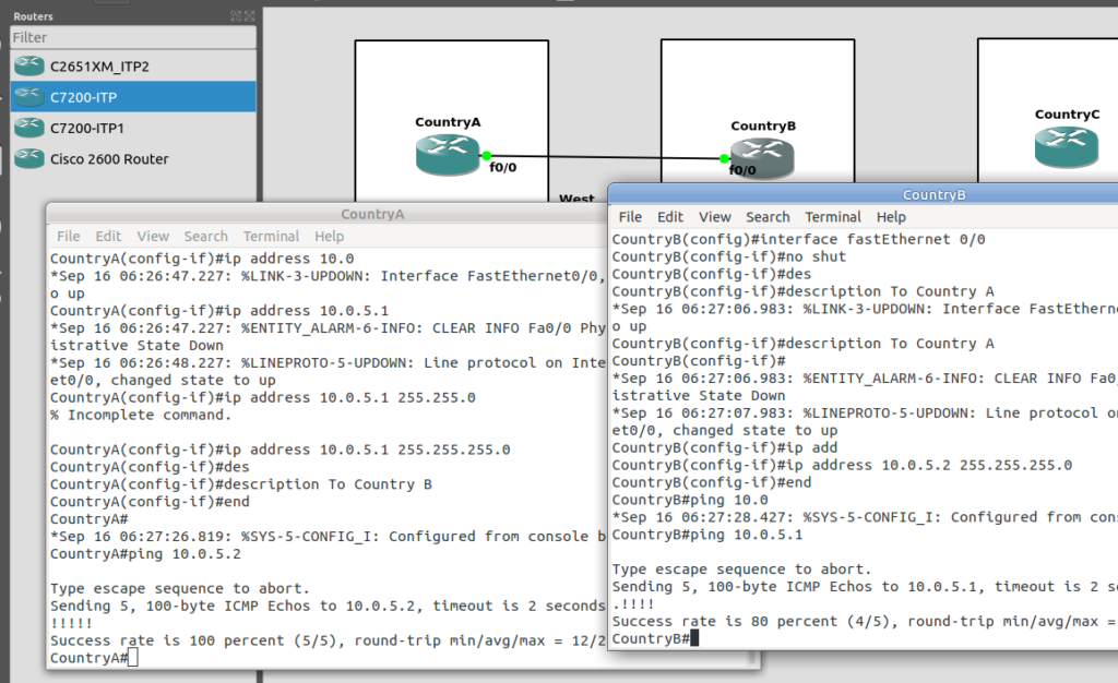
So we’ll configure all the routers in each country with an IP – we don’t need to configure IP routing. This means adjacent countries with a direct connection between them should be able to ping each other, but separated countries shouldn’t be able to.
So now we’ve got IP connectivity between two countries, let’s get Sigtran / SS7 setup!
First we’ll need to define the basics, from configure-terminal in each of the Cisco STPs. We’ll need to set the SS7 variant (We’ll use ITU variant as we’re simulating international links), the network-indicator (This is an International network, so we’ll use that) and the point code for this STP (From the background image).
CountryA(config)#cs7 variant itu
CountryA(config)#cs7 network-indicator international
CountryA(config)#cs7 point-code 1.2.3
Repeat this step on Country A and Country B.
Next we’ll define a local peer on the STP. This is an instance of the Sigtran stack along with the port we’ll be listening on. Our remote peer will need to know this value to bring up the connection, the number specified is the port, and the IP is the IP it will bind on.
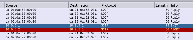
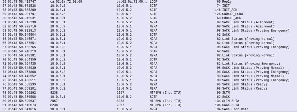
If you’re still sniffing the traffic between Country A and Country B, you should see our SS7 connection come up.
Wireshark trace of the connection coming up
The conneciton will come up layer-by-layer, firstly you’ll see the transport layer (SCTP) bring up an SCTP association, then MTP2 Peer Adaptation Layer (M2PA) will negotiate up to confirm both ends are working, then finally you’ll see MTP3 messaging.
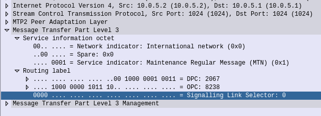
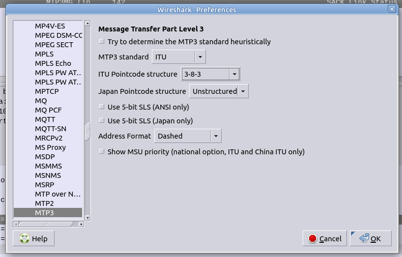
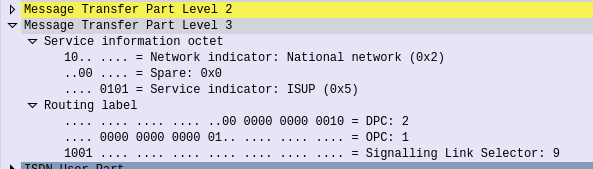
If we open up an MTP3 packet you can see our Originating and Destination Point Codes.
Notice in Wireshark the Point Codes don’t show up as 1-2-3, but rather 2067? That’s because they’re formatted as Decimal rather than 14 bit, this handy converter will translate them for you, or you can just change your preference in Wireshark’s decoders to use the matching ITU POint Code Structure.
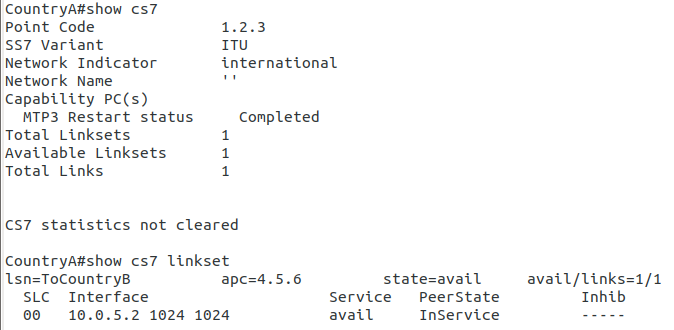
From the CLI on one of the two country STPs we can run some basic commands to view the status of all SS7 components and Linksets.
And there you have it! Basic SS7 connectivity!
There is so much more to learn, and so much more to do! By bringing up the link we’ve barely scratched the surface here.
Some homework before the next post, link all the other countries shown together, with Country D having a link to Country C and Country B. That’s where we’ll start in the lab – Tip: You’ll find you’ll need to configure a new cs7 local-peer for each interface, as each has its own IP.
This is part of a series of posts looking into SS7 and Sigtran networks. We cover some basic theory and then get into the weeds with GNS3 based labs where we will build real SS7/Sigtran based networks and use them to carry traffic.
So one more step before we actually start bringing up SS7 / Sigtran networks, and that’s to get a bit of a closer look at what components make up SS7 networks.
Recap: What is SS7?
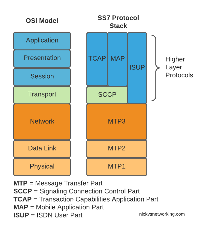
SS7 is the name given to the protocol stack used almost exclusively in the telecommunications space. SS7 isn’t just one protocol, instead it is a suite of protocols. In the same way when someone talks about IP networking, they’re typically not just talking about the IP layer, but the whole stack from transport to application, when we talk about an SS7 network, we’re talking about the whole stack used to carry messages over SS7.
And what is SIGTRAN?
Sigtran is “Signaling Transport”. Historically SS7 was carried over TDM links (Like E1 lines).
As the internet took hold, the “Signaling Transport” working group was formed to put together the standards for carrying SS7 over IP, and the name stuck.
I’ve always thought if I were to become a Mexican Wrestler (which is quite unlikely), my stage name would be DSLAM, but SIGTRAN comes a close second.
Today when people talk about SIGTRAN, they mean “SS7 over IP”.
What is in an SS7 Network?
SS7 Networks only have 3 types of network elements:
Service Switching Points (SSP)
Service Transfer Points (STP)
Service Control Points (SCP)
Service Switching Points (SSP)
Service Switching Points (SSPs) are endpoints in the network. They’re the users of the connectivity, they use it to create and send meaningful messages over the SS7 network, and receive and process messages over the SS7 network.
Like a PC or server are IP endpoints on an IP Network, which send and receive messages over the network, an SSP uses the SS7 network to send and receive messages.
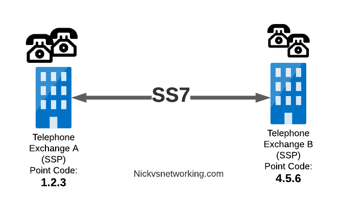
In a PSTN context, your local telephone exchange is most likely an SS7 Service Switching Point (SSP) as it creates traffic on the SS7 network and receives traffic from it.
A call from a user on one exchange to a user on another exchange could go from the SSP in Exchange A, to the SSP in Exchange B, in the same way you could send data between two computers by connecting directly between them with an Ethernet crossover cable.
Messages between our two exchanges are addressed using Point Codes, which can be thought of a lot like IP Addresses, except shorter.
In the MTP3 header of each SS7 message is the Destination Point Code, and the Origin Point Code.
When Telephone Exchange A wants to send a message over SS7 to Telephone Exchange B, the MTP header would look like:
MTP3 Header:
Origin Point Code:      1.2.3
Destination Point Code: 4.5.6
Service Transfer Points (STP)
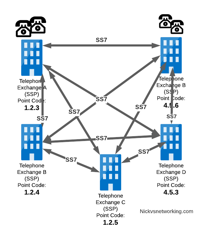
Linking each SSP to each other SSP has a pretty obvious problem as our network grows.
What happens if we’ve got hundreds of SSPs? If we want a full-mesh topology connecting every SSP to every other SSP directly, we’d have a rats nest of links!
A “full-mesh” approach for connecting SSPs does not work at scale, so STPs are introduced
So to keep things clean and scalable, we’ve got Signalling Transfer Points (STPs).
STPs can be thought of like Routers but in an SS7 network.
When our SSP generates an SS7 message, it’s typically handed to an STP which looks at the Destination Point Code, it’s own routing table and routes it off to where it needs to go.
STP acting as a central router to connect lots of SSPs
This means every SSP doesn’t require a connection to every other SSP. Instead by using STPs we can cut down on the complexity of our network.
When Telephone Exchange A wants to send a message over SS7 to Telephone Exchange B, the MTP header would look the same, but the routing table on Telephone Exchange A would be setup to send the requests out the link towards the STP.
MTP3 Header:
Origin Point Code:      1.2.3
Destination Point Code: 4.5.6
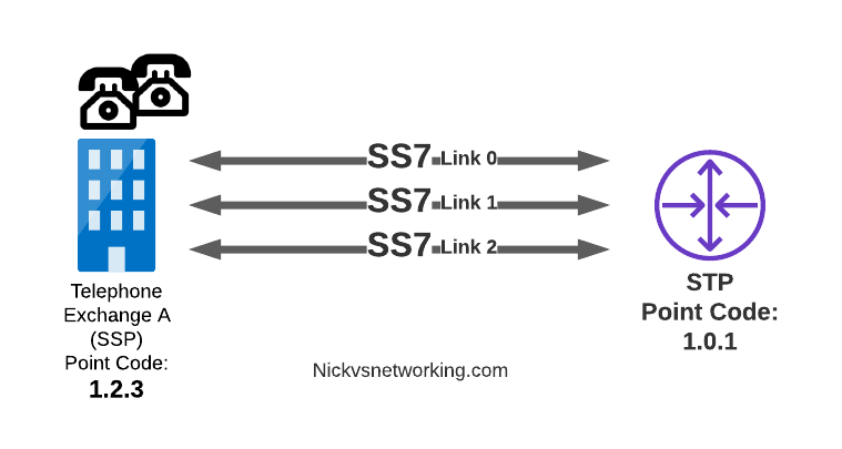
Linksets
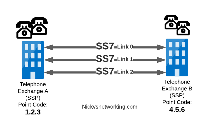
Between SS7 Nodes we have Linksets. Think of Linksets as like LACP or Etherchannel, but for SS7.
You want to have multiple links on every connection, for sharing out the load or for redundancy, and a Linkset is a group of connections from one SS7 node to another, that are logically treated as one link.
Link between an SSP and STP with 3 linksets
Each of the links in a Linkset is identified by a number, and specified in in the MTP3 header’s “Signaling Link Selector” field, so we know what link each message used.
MTP3 Header:
Origin Point Code:       1.2.3
Destination Point Code:  4.5.6
Signaling Link Selector: 2
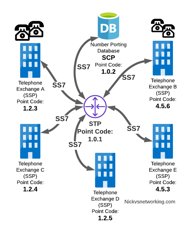
Service Control Point (SCP)
Somewhere between a Rolodex an relational database, is the Service Control Point (SCP).
For an exchange (SSP) to route a call to another exchange, it has to know the point code of the destination Exchange to send the call to. When fixed line networks were first deployed this was fairly straight forward, each exchange had a list of telephone number prefixes and the point code that served each prefix, simple.
But then services like number porting came along when a number could be moved anywhere. Then 1800/0800 numbers where a number had to be translated back to a standard phone number entered the picture.
To deal with this we need a database, somewhere an SSP can go to query some information in a database and get a response back.
This is where we use the Service Control Point (SCP).
Keep in mind that SS7 long predates APIs to easily lookup data from a service, so there was no RESTful option available in the 1980s.
When a caller on a local exchange calls a toll free (1800 or 0800 number depending on where you are) number, the exchange is setup with the Point Code of an SCP to query with the toll free number, and the SCP responds back with the local number to route the call to.
While SCPs are fading away in favor of technology like DNS/ENUM for Local Number Portability or Routing Databases, but they are still widely used in some networks.
Getting to know the Signalling Transfer Point (STP)
As we saw earlier, instead of a one-to-one connection between each SS7 device to every other SS7 device, Signaling Transfer Points (STP) are used, which act like routers for our SS7 traffic.
The STP has an internal routing table made up of the Point Codes it has connections to and some logic to know how to get to each of them.
Like a router, STPs don’t really create SS7 traffic, or consume traffic, they just receive SS7 messages and route them on towards their destination.
Ok, they do create some traffic for checking links are up, etc, but like a router, their main job is getting traffic where it needs to go.
When an STP receives an SS7 message, the STP looks at the MTP3 header. Specifically the Destination Point Code, and finds if it has a path to that Point Code. If it has a route, it forwards the SS7 message on to the next hop.
Like a router, an STP doesn’t really concern itself with anything higher than the MTP3 layer – As point codes are set in the MTP3 layer that’s the only layer the STP looks at and the upper layers aren’t really “any of its business”.
STPs don’t require a direct connection (Linkset) from the Originating Point Code straight to the Destination Point Code. Just like every IP router doesn’t need a direct connection to ever other network. By setting up a routing table of Point Codes and Linksets as the “next-hop”, we can reach Destination Point Codes we don’t have a direct Linkset to by routing between STPs to reach the final Destination Point Code.
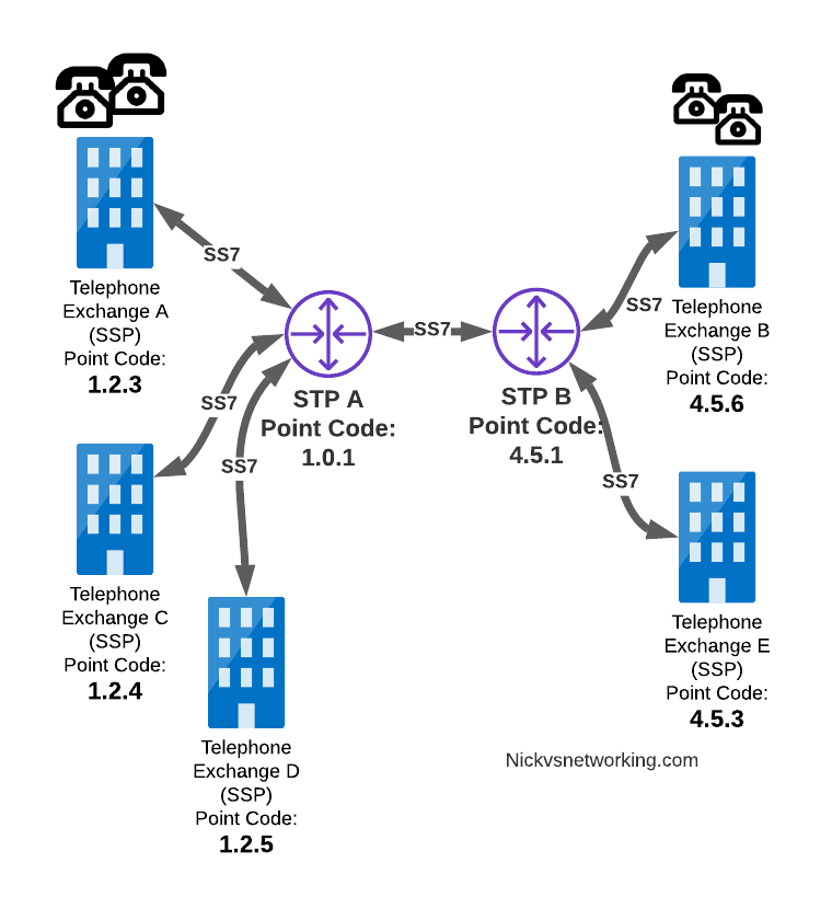
Let’s work through an example:
And let’s look at the routing table setup on STP-A:
STP A Routing Table:
1.2.3 - Directly attached (Telephone Exchange A)
1.2.4 - Directly attached (Telephone Exchange C)
1.2.5 - Directly attached (Telephone Exchange D)
4.5.1 - Directly attached (STP-B)
4.5.3 - Via STP-B
4.5.6 - Via STP-B
So what happens when Telephone Exchange A (Point Code 1.2.3) wants to send a message to Telephone Exchange E (Point Code 4.5.3)? Firstly Telephone Exchange A puts it’s message on an MTP3 payload, and the MTP3 header will look something like this:
MTP3 Header:
Origin Point Code:       1.2.3
Destination Point Code:  4.5.3
Signaling Link Selector: 1
Telephone Exchange A sends the SS7 message to STP A, which looks at the MTP3 header’s Destination Point Code (4.5.3), and then in it’s routing table for a route to the destination point. We can see from our example routing table that STP A has a route to Destination Point Code 4.5.3 via STP-B, so sends it onto STP-B.
For STP-B it has a direct connection (linkset) to Telephone Exchange E (Point Code 4.5.3), so sends it straight on
Like IP, Point Codes have their own form of Variable-Length-Subnet-Routing which means each STP doesn’t need full routing info for every Destination Point Code, but instead can have routes based on part of the point code and a subnet mask.
But unlike IP, there is no BGP or OSPF on SS7 networks. Instead, all routes have to be manually specified.
For STP A to know it can get messages to destinations starting with 4.5.x via STP B, it needs to have this information manually added to it’s route table, and the same for the return routing.
Sigtran & SS7 Over IP
As the world moved towards IP enabled everything, TDM based Sigtran Networks became increasingly expensive to maintain and operate, so a IETF taskforce called SIGTRAN (Signaling Transport) was created to look at ways to move SS7 traffic to IP.
When moving SS7 onto IP, the first layer of SS7 (MTP1) was dropped, as it primarily concerned the physical side of the network. MTP2 didn’t really fit onto an IP model, so a two options were introduced for transport of the MTP2 data, M2PA (Message Transfer Part 2 User Peer-to-Peer Adaptation Layer) and M2UA (MTP2 User Adaptation Layer) were introduced, which rides on top of SCTP. This means if you wanted an MTP2 layer over IP, you could use M2UA or M2TP.
SCTP is neither TCP or UDP. I’ve touched upon SCTP on this blog before, it’s as if you took the best bits of TCP without the issues like head of line blocking and added multi-homing of connections.
So if you thought all the layers above MTP2 are just transferred, unchanged on top of our M2PA layer, that’s one way of doing it, however it’s not the only way of doing it.
There are quite a few ways to map SS7 onto IP Networks, which we’ll start to look into it more detail, but to keep it simple, for the next few posts we’ll be assuming that everything above MTP2/M2PA remain unchanged.
In the next post, we’ll get some actual SS7 traffic flowing!
This is part of a series of posts looking into SS7 and Sigtran networks. We cover some basic theory and then get into the weeds with GNS3 based labs where we will build real SS7/Sigtran based networks and use them to carry traffic.
If you use a mobile phone, a VoIP system or a copper POTS line, there’s a high chance that somewhere in the background, SS7 based signaling is being used.
The signaling for GSM, UMTS and WCDMA mobile networks all rely on SS7 based signaling, and even today the backbone of most PSTN traffic relies SS7 networks. To many this is mysterious carrier tech, and as such doesn’t get much attention, but throughout this series of posts we’ll take a hands-on approach to putting together an SS7 network using GNS3 based labs and connect devices through SS7 and make some stuff happen.
Overview of SS7
Signaling System No. 7 (SS7/C7) is the name for a family of protocols originally designed for signaling between telephone switches. In plain English, this means it was used to setup and teardown large volumes of calls, between exchanges or carriers.
When carrier A and Carrier B want to send calls between each other, there’s a good chance they’re doing it over an SS7 Network.
But wait! SIP exists and is very popular, why doesn’t everyone just use SIP? Good question, imaginary asker. The answer is that when SS7 came along, SIP was still almost 25 years away from being defined. Yes. It’s pretty old.
SS7 isn’t one protocol, but a family of protocols that all work together – A “protocol stack”. The SS7 specs define the lower layers and a choice of upper layer / application protocols that can be carried by them.
The layered architecture means that the application layer at the top can be changed, while the underlying layers are essentially the same.
This means while SS7’s original use was for setting up and tearing down phone calls, this is only one application for SS7 based networks. Today SS7 is used heavily in 2G/3G mobile networks for connectivity between core network elements in the circuit-switched domain, for international roaming between carriers and services like Local Number Portability and Toll Free numbers.
Here’s the layers of SS7 loosely mapped onto the OSI model (SS7 predates the OSI model as well):
OSI Model (Left) and SS7 Protocol Stack (Right)
We do have a few layers to play with here, and we’ll get into them all in depth as we go along, but a brief introduction to the underlying layers:
MTP 1 – Message Transfer Part 1
This is our physical layer. In this past this was commonly E1/T1 lines.
It’s responsible for getting our 1s and 0s from one place to another.
MTP 2 – Message Transfer Part 2
MTP2 is responsible for the data link layer, handling reliable transfer of data, in sequence.
MTP 3 – Message Transfer Part 3
The MTP3 header contains an Originating and a Destination Point Code.
These point codes can be thought of as like an IP Address; they’re used to address the source and destination of a message. A “Point Code” is the unique address of a SS7 Network element.
MTP3 header showing the Destination Point Code (DPC) and Origin Point Code (OPC) on a National Network, carrying ISUP traffic
Every message sent over an SS7 network will contain an Origin Point Code that identifies the sender, and a Destination Point Code that identifies the intended recipient.
This is where we’ll bash around at the start of this course, setting up Linksets to allow different devices talking to each other and addressing each other via Point Codes.
The MTP3 header also has a Service Indicator flag that indicates what the upper layer protocol it is carrying is, like the Protocol indicator in IPv4/IPv6 headers.
A Signaling Link Selector indicates which link it was transported over (did I mention we can join multiple links together?), and a Network Indicator for determining if this is signaling is at the National or International level.
TUP/MAP/SCCP/ISUP
These are the “higher-layer” protocols. Like FTP sits on top of TCP/IP, a SS7 network can transport these protocols from their source to their destination, as identified by the Origin Point Code (OPC), to the Destination Point Code (DPC), as specified in the MTP3 header.
We’ll touch on these protocols more as we go on. SCCP has it’s own addressing on top of the OPC/DPC (Like IP has IP Addressing, but TCP has port numbers on top to further differentiate).
Why learn SS7 today?
SS7 and SIGTRAN are still widely in use in the telco world, some of it directly, other parts derived / evolved from it.
So stick around, things are about to get interesting!
So I’ve been waxing lyrical about how cool in the NRF is, but what about how it’s secured?
A matchmaking service for service-consuming NFs to find service-producing NFs makes integration between them a doddle, but also opens up all sorts of attack vectors.
Theoretical Nasty Attacks (PoC or GTFO)
Sniffing Signaling Traffic: A malicious actor could register a fake UDR service with a higher priority with the NRF. This would mean UDR service consumers (Like the AUSF or UDM) would send everything to our fake UDR, which could then proxy all the requests to the real UDR which has a lower priority, all while sniffing all the traffic.
Stealing SIM Credentials: Brute forcing the SUPI/IMSI range on a UDR would allow the SIM Card Crypto values (K/OP/Private Keys) to be extracted.
Sniffing User Traffic: A dodgy SMF could select an attacker-controlled / run UPF to sniff all the user traffic that flows through it.
Obviously there’s a lot more scope for attack by putting nefarious data into the NRF, or querying it for data gathering, and I’ll see if I can put together some examples in the future, but you get the idea of the mischief that could be managed through the NRF.
This means it’s pretty important to secure it.
OAuth2
3GPP selected to use common industry standards for HTTP Auth, including OAuth2 (Clearly lessons were learned from COMP128 all those years ago), however OAuth2 is optional, and not integrated as you might expect. There’s a little bit to it, but you can expect to see a post on the topic in the next few weeks.
3GPP Security Recommendations
So how do we secure the NRF from bad actors?
Well, there’s 3 options according to 3GPP:
Option 1 – Mutual TLS
Where the Client (NF) and the Server (NRF) share the same TLS info to communicate.
This is a pretty standard mechanism to use for securing communications, but the reliance on issuing certificates and distributing them is often done poorly and there is no way to ensure the person with the certificate, is the person the certificate was issued to.
3GPP have not specified a mechanism for issuing and securely distributing certificates to NFs.
Option 2 – Network Domain Security (NDS)
Split the network traffic on a logical level (VLANs / VRFs, etc) so only NFs can access the NRF.
Essentially it’s logical network segregation.
Option 3 – Physical Security
Split the network like in NDS but a physical layer, so the physical cables essentially run point-to-point from NF to NRF.
NRF and NF shall authenticate each other during discovery, registration, and access token request. If the PLMN uses protection at the transport layer as described in clause 13.1, authentication provided by the transport layer protection solution shall be used for mutual authentication of the NRF and NF. If the PLMN does not use protection at the transport layer, mutual authentication of NRF and NF may be implicit by NDS/IP or physical security (see clause 13.1). When NRF receives message from unauthenticated NF, NRF shall support error handling, and may send back an error message. The same procedure shall be applied vice versa. After successful authentication between NRF and NF, the NRF shall decide whether the NF is authorized to perform discovery and registration. In the non-roaming scenario, the NRF authorizes the Nnrf_NFDiscovery_Request based on the profile of the expected NF/NF service and the type of the NF service consumer, as described in clause 4.17.4 of TS23.502 [8].In the roaming scenario, the NRF of the NF Service Provider shall authorize the Nnrf_NFDiscovery_Request based on the profile of the expected NF/NF Service, the type of the NF service consumer and the serving network ID. If the NRF finds NF service consumer is not allowed to discover the expected NF instances(s) as described in clause 4.17.4 of TS 23.502[8], NRF shall support error handling, and may send back an error message. NOTE 1: When a NF accesses any services (i.e. register, discover or request access token) provided by the NRF , the OAuth 2.0 access token for authorization between the NF and the NRF is not needed.
TS 133 501 – 13.3.1 Authentication and authorization between network functions and the NRF