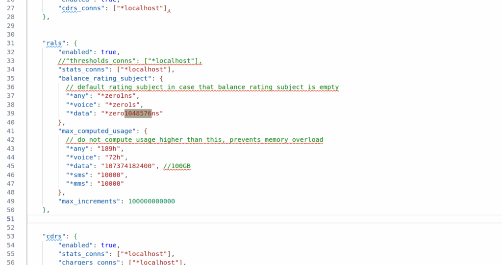
Well CGrateS deducts for each incriment in the usage, and in my case, a usage of 107374182 meant CGrateS was trying to deduct from the balance 107 million times.
But as you can imagine, we don’t actually charge our customers per byte but rather we round up our incriments.
This is where the RatingSubject comes into play. RatingSubject sets what “blocks” of balance get calculated.
For example rather than calculating usage of 107,374,182 bytes, with CGrateS deducting from the balance 107 million times, we could set the value *zero1048576ns which means we’d calculate per Megabyte, so we’re only calculating 102 times 1 megabyte.
Likewise we could set the RatingSubject value to *zero1024ns to get it in Kilobytes.
What’s with the ns suffix? Well CGrateS (actually Go) treats units as duration, and the smallest unit is nanoseconds, but we can ignore the meaning in this context, as just 1 integer unit.
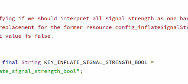
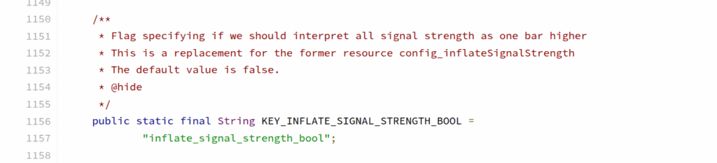
Poking around in Android the other day I found this nugget in Carrier Config manager; a flag (KEY_INFLATE_SIGNAL_STRENGTH_BOOL) to always report the signal strength to the user as one bar higher than it really is.
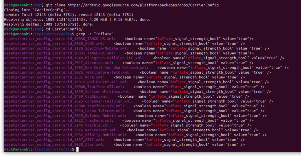
Notably both AT&T and Verizon have this flag enabled on their networks, I’m not sure who was responsible for requesting this to be added to Android, nor could I find it in the git-blame, but we can see it in the CarrierConfig which contains all the network settings for each of these operators.
Operators are always claiming to have the biggest coverage or the best network, but stuff like this, along with the fake 5G flags, don’t help build trust, especially considering the magic mobile phone antennas which negate the need for all this deception anyway.
We were testing international roaming for a customer, roaming into the US where one of our team members (shoutout to Cody) is based.
So we sent Cody some SIMs and asked them to run the basic tests for us, but no IMS APN would attach.
We’d get them to power up the phone, fire up a trace on the roaming PGWs, but never seeing an attempt to attach on the IMS APN (No Create Session Request from the SGW in the vPMN).
The operator we were roaming into swore their side was correct – that IMSI was allowed for the IMS APN for testing, but whenever we’d run a trace, same thing, default bearer just fine but no CSR for the IMS APN, as if the IMS APN was blocked on the roaming network (Which is common on networks where you haven’t launched VoLTE but do have data roaming).
The steps we would do is:
Person in the US turns on phone tries to attach
I fire up my computer, get a trace running
Person in the US airplanes the device
I monitor for CSRs on the PGWs for that IMSI
But no CSR for the IMS APN would ever come through.
After a few attempts, here’s what we found was happening:
The phone would get powered up
The phone would roam onto the vPMN in the US and the default bearer would come up
The phone would try to attach to the ims APN, this would work for this SIM which was whitelisted, and the Create Session Request for the ims APN went to the PGW in the hPMN
The ims APN came up as expected
The phone would send a SIP REGISTER (So far so good)
Our IMS had an issue with Rx routing in this scenario, so the SIP REGISTER would timeout, and when it timed out, a 504 error was sent back to the phone by the P-CSCF and it set the Retry-After header to 3600 seconds.
The phone would not try again for as long as that timer value was set.
At this point we’d start a trace, airplane the device, and see no IMS APN attach attempt.
This 504 Timeout would all happen when the phone fired up before we had any traces running, so we weren’t capturing that.
I’d wrongly assumed that airplaning the device after starting a trace would reset the state fully, but it doesn’t, neither does a restart of the phone.
When we’d started a trace and airplane the phone, the phone wouldn’t try to attach to the ims APN as it was still inside the Retry-After time window from when we’d first fired it up.
Per RFC 3261, the phone should not try again during this time, which in our case meant no attempt to attach to the IMS APN, this makes sense – it protects the network against the thundering herd problem, but made this otherwise simple fault really hard to find.
Recently I’ve been playing with creating UPPs – Unprotected Profile Packages – The “profile” that gets loaded onto eSIMs.
While that’s worthy of a post itself, for testing I’ve found it really convenient to be able to “explore” the created SIM profile in PySIM, Gemalto Card Admin, etc, and check the behavior in a real handset using the SIMtrace.
So how do you get an eSIM onto a physical card?
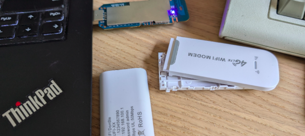
For that I’m using a physical consumer eSIM, which is a physical SIM card I can load an eSIM onto.
Normally the eSIM is baked into your phone, but this one isn’t, it’s baked into a 4FF form factor.
But while iOS and Android have got flows for loading the eSIM (the Local Profile Assistant), this is just a bit of plastic, so we need our own external LPA to pull the eSIM from the SM-DP+ and load it onto the card.
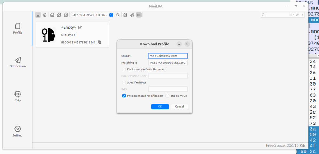
So in addition to this a SIM card reader I used a nifty util called MiniLPA which is the Local-Profile-Assistant, used to load eSIM profiles onto the eSIM itself.
I installed the Debian package of MiniLPA, started it up, plugged in my SIM reader and consume eUICC, then took the LPA address and split the SM-DP+ address (the Domain name part) and the ID (the long hex string part) up and plugged them into the download profile window and boom, I had a profile loaded and could work with the eSIM profile on a physical card.
The Network Repository Function is essentially a database used to store/query information about NFs on the network.
To do this, the NRF has 3 services: the Nnrf_NFManagement Service is used to insert/update/remove records into the database of NFs on the network, the Nrf_NFDiscovery service is used to query this database, and the OAuth2 Authorization service is used to authenticate / authorize the transactions of the first two securely.
The Nnrf_NFManagement Service
The Nnrf_NFManagement Service is the service that handles the registration, deregistration and updating the database of service-producing NFs.
When a NF offering a service becomes ready for service, it registers with the NRF to advise the NRF of the services it offers and so service-consumers (Clients) are able to find and then request services from this NF.
Let’s take a look at the NFRegister process, which is the service operation used to register an NF in the NRF.
At its heart, the NFRegister process is a HTTP2 PUT sent from the NF to the NRF to the path <nrf_ip>/nnrf-nfm/v1/nf-instances/{nrf-instance-id} with a JSON payload containing all the specifics of the services being offered by the NF (NFProfile), which is sent to the NRF.
The NRF parses through the message body (That JSON Payload containing the NFProfile) and adds all this info to the internal database in the NRF as to which service producers it has available.
If this is all OK from the NRF’s perspective, then a 200 OK is sent back by the NRF.
The NFProfile JSON body
The NFProfile is a JSON encoded message body that contains all the info about the NF that the NRF takes and adds to its internal database of services offered by that NF.
nfInstanceID – The Network Function Instance ID is the unique identity if this NF. (It’s also included in the Request URI) It’s a unique ID and typically generated randomly by the NF itself.
nfType – The type of the NF itself, there’s a long list of supported NF Types, NRF, UDM, AMF, SMF, AUSF, etc, etc.
nfStatus – Is the status of the NF, either REGISTERED (Discoverable by other NFs), SUSPENDED (Registered in the NRF but not able to be discovered / invisible, NFs in this state are usually here because they’ve had a high failure rate or haven’t been responding to heartbeats), UNDISCOVERABLE (Used when an NF wants to stop offering services to new consumers, but is still able to offer services to existing consumers, the idea being this is taking it out of the discovery pool, but still able to serve in-process requests).
plmnList – This is a list of PLMNs that this NF serves.
fqdn – The Fully Qualified Domain name of the NF
IPv4Address / IPv6Address – The IPv4 and/or IPv6 address of the NF
nfService – This is a list of JSON objects, detailing the services offered by the NF, such as the service names it is offering, version of the service, IDs of the service instances and IP Endpoints for requests to be sent to.
priority / capacity / load – Used for selection of this NF from the pool and the order of results returned
The Nnrf_NFManagement Service also includes a Subscription service, to allow NFs to subscribe to changes in state, for example getting a notification if a NF that was registered becomes deregistered.
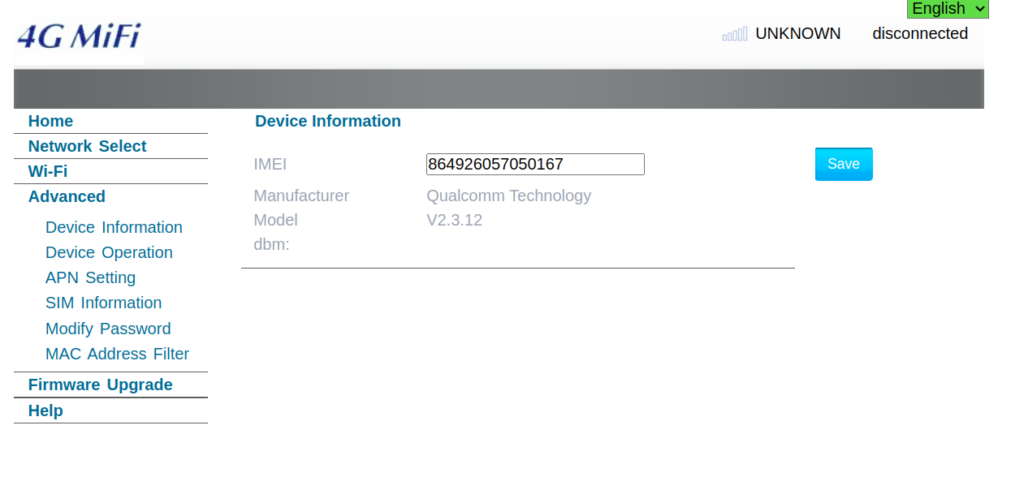
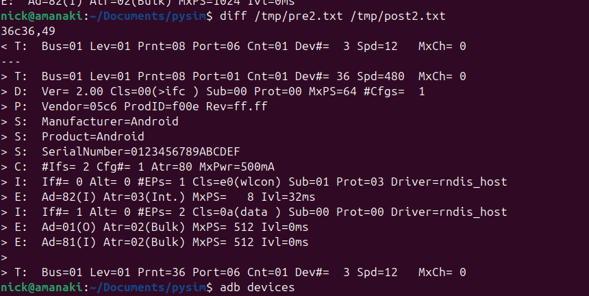
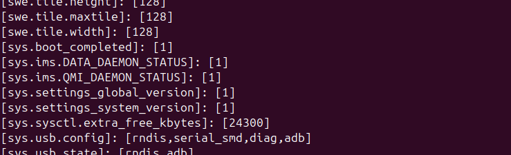
The device showed up as an rndis_host adapter in Linux, just like a USB NIC, and browsing to the default gateway shows a web UI where amazingly, you can set the IMEI – Pretty sure this isn’t legal…
This is not the IMEI it came with – that’s the IMEI of a EP06-e chip on my desk…
Oddly I could see it was an Android device, but with no adb port exposed, but wait – does that mean this an Android phone in a USB stick?
Alas no DIAG mode serial adapter showed up, despite a few variations on the above.
So with ADB connected could I stream the video from the device and use it like an Android phone?
You betcha:
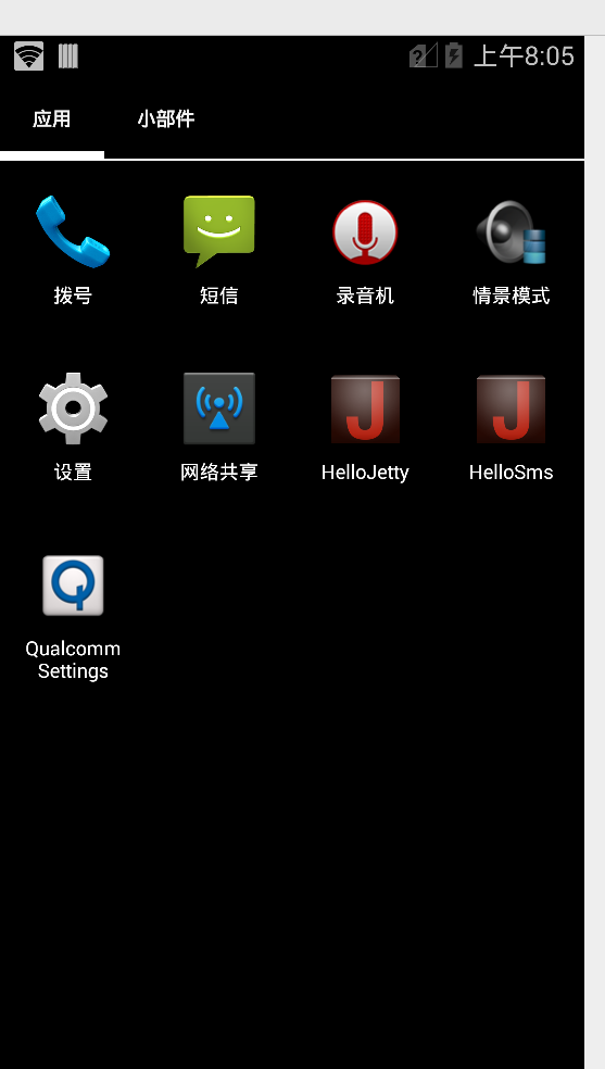
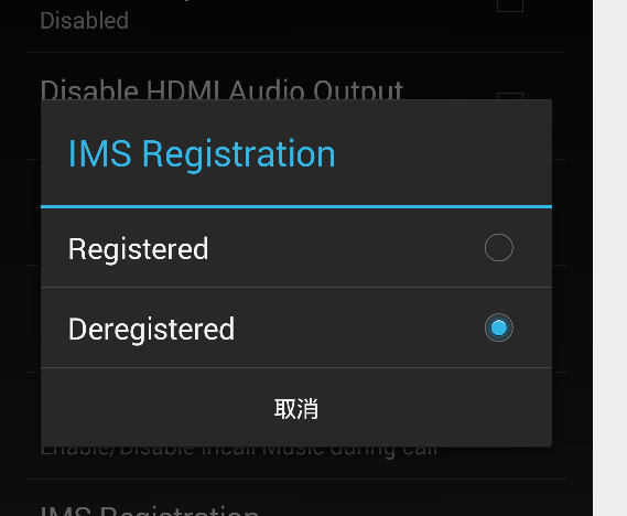
After poking around in Android I found an App called “Qualcomm Settings” which piqued my interest.
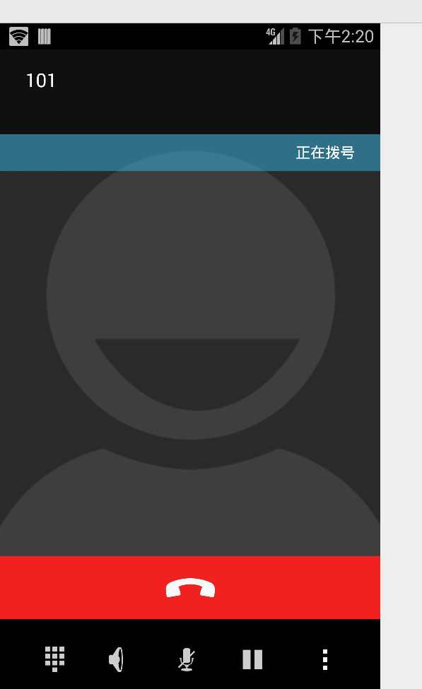
Alas the unit only supports LTE Band 1 / 3 / 5 none of which I have in my office (I’m too lazy to go out to the lab to fire up an Airscale) so I put a public SIM in it and was able to use data, but when I tried to make a call it seems it kicked off CS fallback.
More exploring to do, but pretty amazing what $10 buys you!
So we’ve found this scenario that occurs on some Samsung UEs, in certain radio contions, where midway through an otherwise normal voice call, the UE sends “mystery” data (Not IP data), which in turn causes the UPF to send the error indication and drop the bearer, which in turn drops the call.
The call starts, like any normal call, SIP REGISTER, INVITE, etc.
The P-CSCF / PCRF / PGW set up the dedicated bearer for the voice traffic, and the RTP stream starts flowing over it.
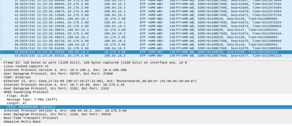
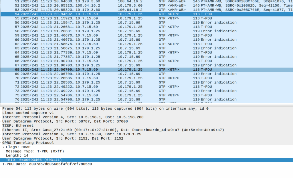
Then the UE sends these weird packets instead of the RTP stream:
These are GTP-U encapsulated data, with the TEID that matches the TEID used for the RTP stream, but there’s no IP data in them – they’re only 14 bytes long and sent by the UE.
Here’s some examples of what’s sent (each line is a packet):
An IPv4 header is 20 bytes long, and IPv6 header is 40, so this is too short for either of those protocols, but what else could it be?
There’s some commonality of course, starts d0 as the first octet, then d1, d2, d3, etc. So that’s something?
I thought perhaps it was a boundary issue, that the standard RTP packet was being split across multiple GTP-U payloads, but that doesn’t appear to be the case.
An Ethernet header is 14 bytes, but if we were to decode this as Ethernet there’s still nothing it’s transporting, and the destination MAC is changing sequentailly if that’s the case, which would be even weirder.
I also thought about RTP that for some reason has lost it’s IP/UDP header, as the sequentially counting byte at the start could be the RTP sequence number, but that’d be 19 bytes minimum and the sequence number is the 3rd and 4th byte, not the first.
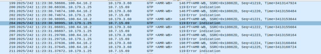
Whatever they contain, we see this sent over and over for a few seconds, then bam, back to normal RTP stream flowing.
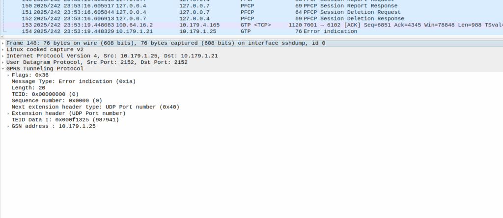
Or at least it should be, but the invalid packet causes the UPF to generate a GTP-U Error Indication.
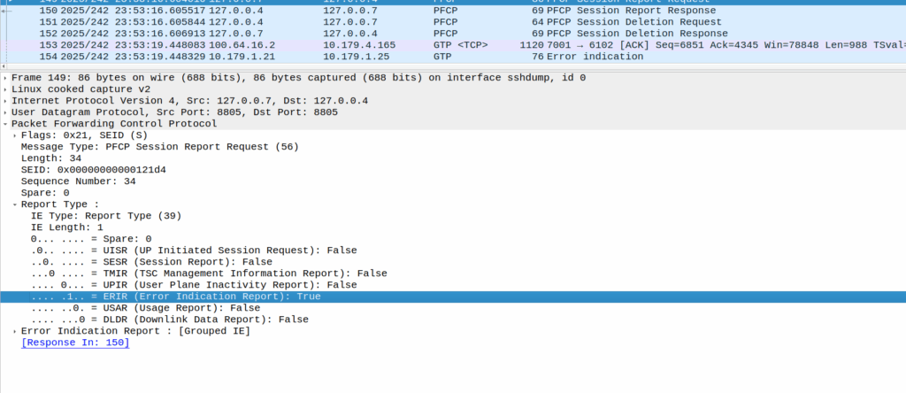
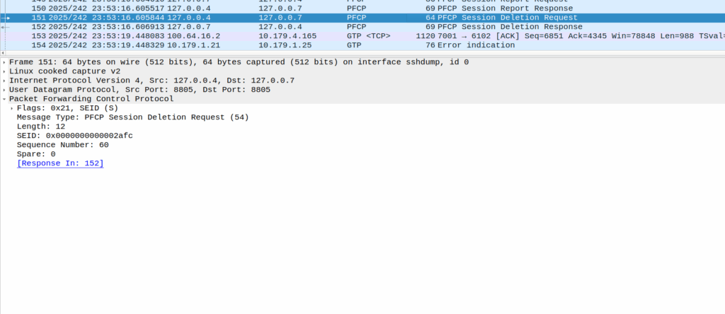
These Error Indication payloads eventually lead to the next PFCP Session Report Request having the Error Indication Report (ERIR) flag set to True.
When the PGW-U gets this, it sends a Session Delete Request, which dutifully drops the bearer.
Meaning the session drops on the EPC side, and the RTP drops with it, eventually a BYE is sent from the phone due to RTP timeout.
The above screenshot shows a different cause of GTP-U Error Indication – At this point the bearer has been dropped on the EPC side and these are Error Indications to report it doesn’t know the TIED / bearer.
How to fix this?
Well, unlikely we’ll get a fix on the Samsung side, so we’ll need to not drop the bearer on the PGW-C if we get a lot of Error Indications, and hope for the best.
The UE Authentication Service is consumed by the AMF. The AMF initiates the authentication operation, when indicated, as part of the UE registration process. The AUSF performs either 5G-AKA or EAP-based authentication based on information received from the AMF. If EAP authentication is used then the AUSF and the UE exchange EAP messages through the AMF.
3GPP TS 29.509 V16.3.0; 5G System; Authentication Server Services
Common Dialogs on Nausf-auth Service
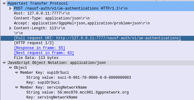
Authenticate UE – Request
HTTP POST sent from the AMF to the AUSF, to the URL /nausf-auth/v1/ue-authentications with JSON body containing the SUPI or the SUCI, and the serving network name.
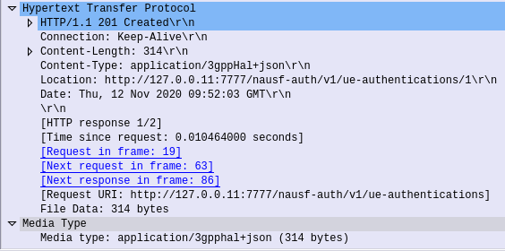
Authenticate UE – Response
If request from the AMF is successfully processed by the AUSF, it sends back a “201 Created” response, with a JSON Body containing the authentication vectors:
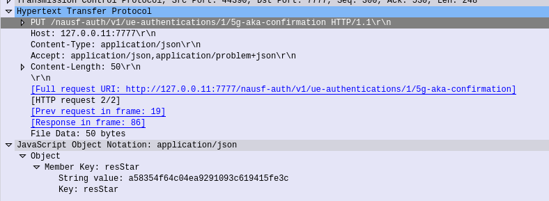
The AMF needs to advise the AUSF the RES returned from the Subscriber (if one was returned) to confirm the UE successfully authenticated, so the AMF sends this in the form of an HTTP PUT to the AUSF to the URL /nausf-auth/v1/ue-authentications/1/5g-aka-confirmation
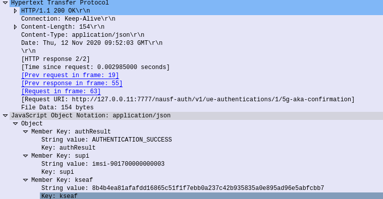
5G-AKA Confirmation – Response
If successful a 200 OK is sent back to the AMF by the AUSF with a JSON body containing the SUPI of the Subscriber (keep in mind the subscriber may have authenticated with a SUCI, so up until this point the AMF doesn’t know the SUPI of the Subscriber), and the Kseaf key used for ciphering and integrity protection.
Common Dialogs on Nudm-ueau Service
The Nudm_UEAuthentication service is used by NF service consumers to obtain UE authentication vectors from the UDM, to inform the UDM of authentication results, to query authentication results, and to purge authentication results.
3GPP TS 29.503 Unified Data Management Services
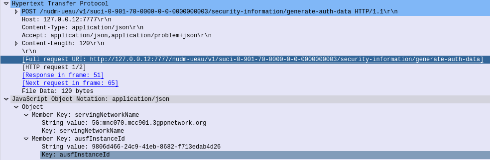
Generate Authentication Data – Request
When the AUSF needs to authenticate a subscriber, for example because an AMF has requested vectors, it in turn needs to request this information be generated by the UDM.
So the AUSF sends a HTTP POST to /nudm-ueau/v1/suci-0-901-70-0000-0-0-0000000003/security-information/generate-auth-data on the UDM (Where 901-70-0000-0-0-0000000003 is the SUPI or SUCI of the subscriber), and with a JSON body containing the AUSF’s Instance ID.
Generate Authentication Data – Response
Once the UDM has
The UDM will need to take the SUPI/SUCI provided by the AUSF and generate the authentication vectors following the AKA Process taking the OP/OPc & K keys as inputs.
The UDM sends a 200 OK back to the AUSF that requested the information, with a JSON Body containing the full vectors, including the Kausf to be provided to the AMF when the subscriber has successfully authenticated.
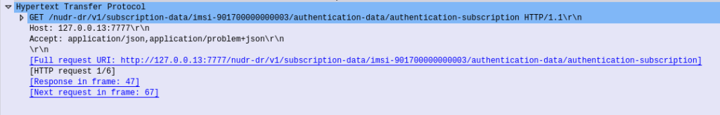
The AUSF sends an HTTP GET to the UDM with the SUPI/SUCI in the URI /nudr-dr/v1/subscription-data/imsi-901700000000003/authentication-data/authentication-subscription
To do this the UDM needs the K & OP (or OPc) values for that subscriber, depending on the UDM configuration, it may have this data cached, or it may need to retrieve these values from the UDR.
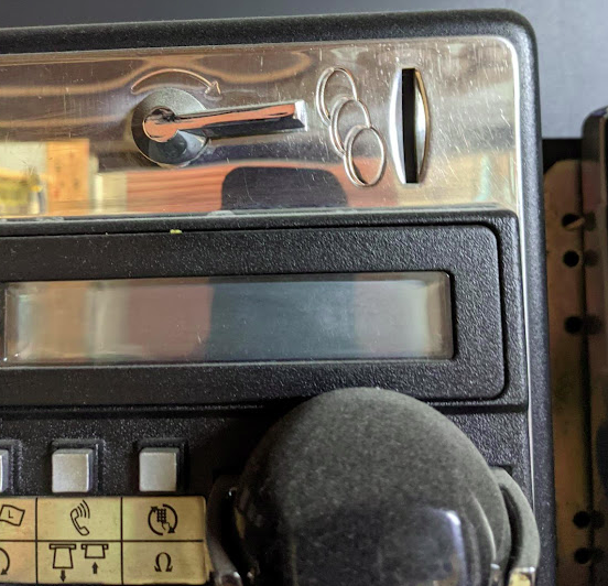
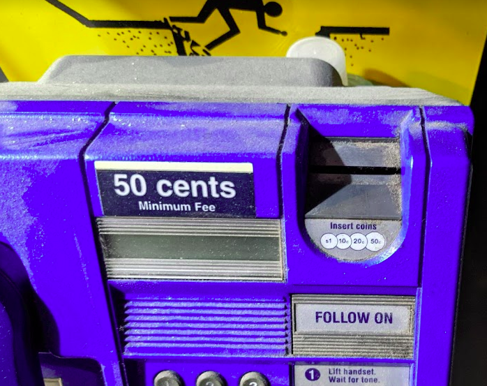
Let’s imagine the coin slot on a payphone – Coins can only enter the slot if they’re aligned with the slot.
If you tried to rotate the coin by 90 degrees, it wouldn’t fit it in the slot.
If the slot on the payphone went from up-to-down, our coin slot could be described as “vertically polarized”. Only coins in the vertically polarized orientation would fit.
Likewise, a payphone with the coin slot going side-to-side we could describe the coin slot as being “horizontally polarized”, meaning only coins that are horizontally polarized (on their side) would fit into the coin slot.
RF waves also have a polarization, like our coin slot.
A receiver wishing to receive into signals transmitted from a vertically-polarized antenna, will need to use a vertically-polarised antenna to pick up the signal.
Likewise a signal transmitted from a horizontally polarized antenna, would require a horizontally polarised antenna on the receiving side.
If there is a mismatch in polarization (for example RF waves transmitted from a horizontal polarized antenna but the receiver is using a vertically polarized antenna) the signal may still get through, but received signal strength would be severely degraded – in the order of 20dB, which is 1/100th of the power you’d get with the correct polarization.
You can think of polarization mismatches as like cutting up the coin to fit sideways through the coin slot – you’d get a sliver of the original coin that was cut up to fit. Much like you recieve a fraction of the original signal if your polarization doesn’t match on both ends.
Plagiarised diagram showing antenna polarization
Useless Information: In Australia country TV stations and metro TV stations sometimes transmitted different programming. To differentiate the signals on the receiver side, country TV transmitters used vertical polarisation, while metro transmitters used horizontal polarization. The use of different polarization orientation cuts down on interference in the border areas that sit in the footprint of the metro and country transmitters. This means as you drive through metro areas you’ll see all the yagi-antennas are horizontally oriented, while in country areas, they’re vertically oriented.
Vertical Polarization
Early mobile phone networks used Vertical Polarization.
This means they used an flagpole like antenna that is vertically oriented (Omnidirectional antenna) on the base-station sites.
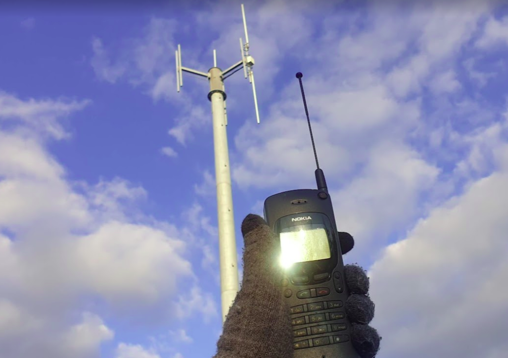
Oldschool mobile phones also had a little pop out omnidirectional antenna, which when you held the phone to your ear, would orient the antenna vertically.
This matches with the antenna on the base station, and away we go. You still sometimes see vertical polarization in use on base-station sites in low density areas, or small cells.
Vertically polarized mobile phone antenna, which is oriented vertically, like on the base station behind it.
Increasing subscriber demand meant that operators needed more capacity in the network, but spectrum is expensive. As we just saw a mismatch in polarization can lead to a huge reduction in power, and maybe we can use that to our advantage…
Shannon-Hartley Theorem
But first, we need to do some maths…
Stick with me, this won’t be that hard to understand I promise.
There are two factors that influence the capacity of a network, the Bandwidth of the Channel and the Signal-to-Noise Ratio.
So let’s look at what each of these terms mean.
Bandwidth
Bandwidth is the information carrying capacity. A one-page sheet of A4 at 12 point font, has a set bandwidth. There’s only so much text you can fit on one A4 sheet at that font size.
A4 Sheet, 12 point font, has 989 words.
We can increase the bandwidth two ways:
Option 1 to Increase Bandwidth: Get a larger transmission medium. Changing the size of the medium we’re working with, we can increase how much data we can transfer.
For this example we could get a bigger sheet of paper, for example an A3 sheet, or a billboard, will give us a lot more bandwidth (content carrying capability) than our sheet of A4.
Changing from an A4 sheet to an A3 sheet, increases the number of characters we can store on the page (Slightly more than doubling the bandwidth).
Option 2 to Increase Bandwidth: Use more efficient encoding As well as changing the size of the medium we are using, we can change how we store the data on the paper, for example, shrinking the font size to get more text in the same area, which also the bandwidth.
In communications networks this is also true: Bandwidth is determined by how much spectrum we have to work with (For example 10Mhz), and how we encode the data on that spectrum, ie morse-code, Binary-Phase-Shift-Keying or 16-QAM. Each of the different encoding schemes have different levels of bandwidth for the same amount of spectrum used, and we’ll cover those in more detail in the future.
So now we’ve covered increasing the bandwidth, now let’s talk about the other factor:
Signal-to-Noise Ratio
Signal-to-NoiseRatio (SNR) is the ratio of good signal, to the background noise.
On the train my headphones on block out most of the other sounds. In this scenario, the signal (the podcast I’m listening to on the headphones) is quite high, compared to the noise (unwanted sounds of other people on the train), so I have a good Signal-to-Noise ratio.
When we talk about the Signal-to-Noise Ratio, we’re talking about the ratio of the signal we want (podcast) to the noise (signal we don’t want).
When I’m on the train if 90% of what I hear is the podcast I’m listening to (the “signal”) and 10% is random background sounds (the “noise”) then my signal-to-noise-ratio is really good (high).
Capacity and SNR
Let’s continue with the listening to a podcast analogy.
The average human talks about 150 words per minute. So let’s imagine I’m listening to a podcast at 150 words per minute.
If I’m listening in an anechoic chamber, then I’ll be able to hear everything that’s being said, so my bandwidth will 150 words per minute. As there is no background noise, my capacity will also be 150 words per minute.
But if I leave an anechoic chamber (much as I love spending time in anechoic chambers), and go back on the train, I won’t hear the full 150 words per minute (bandwidth) due to the noise on the train drowning out some of the signal (podcast).
The Shannon-Hartley Theorem, states that the capacity is equal to the bandwidth multiplied by the signal to noise ratio.
So on the train hearing 90% of what’s said on the podcast, 10% drowned out, means my signal-to-noise ratio is 0.9 (pretty good).
So according to Shannon-Hartley Theorem the capacity of me listening to a podcast on the train (150 words per minute of bandwidth multiplied by 0.9 Signal-to-Noise Ratio) would give me 135 words per minute of capacity.
Claude Shannon, of 1/2 of the Shannon-Hartley Theorem, with an electromechanical mouse maze.
How this applies to RF Networks
In an RF context, our Bandwidth has a fixed information carrying capacity, for example on LTE, with a 5Mhz wide channel using 16QAM has 12.5Mbps of bandwidth available.
In a simple system, we have two levers we can pull to increase the bandwidth:
Increasing the size of the channel – If we went from a 5Mhz wide channel to a 20Mhz channel, this would give us 4x the available Bandwidth (Actually slightly more in LTE, but whatever)
Changing the encoding to cram more data on the same a size channel (From 16QAM to 64QAM would also give us 4x the available Bandwidth).
As we’ll see later in this post, there are some extra tricks (MIMO and Diversity) that we’ll look at later in this post, to increase the bandwidth of the system.
Our Signal-To-Noise (SNR) is constantly variable with a gazillion things that can influence the result. Some of the key factors that impact the SNR are the distance from the transmitter to the receiver and anything blocking the path between them (trees, buildings, mountains, etc), but there’s so many other factors that go into this. From atmospheric conditions, flat surfaces the signal can reflect off leading to multipath noise, other nearby transmitters, etc, can all influence our SNR.
Our capacity is equal to our Bandwidth multiplied by the Signal-to-Noise ratio.
Shannon-Hartley Theorem (ish)
As a goal we want capacity, and in an ideal world, our capacity would be equal to our bandwidth, but all that noise sneaks in and reduces our available capacity, based on the current SNR value.
So now we want to get more capacity out of the network, because everyone always wants to add capacity to networks.
One trick that we can use it to use multiple antennas with different polarization.
If our transmitter sends the same signal data out multiple antennas, with some clever processing on the transmitter and the receiver, we use this to maximize the received SNR. This is called Transmit Diversity and Receive Diversity and it’s a form of black magic.
The Transmitter uses feedback from the receiver to determine what the channel conditions are like, and then before transmitting the next block of data, compensates for the channel conditions experienced by the receiver, this increases the SNR and allows for higher MCS / encoding schemes, which in turns means higher throughput.
You’ll notice on most Antennas in the wild today you’ve got at least two ports for each frequency, which are + and -, which are the two polarizations.
Modern mobile networks use ±45° slant polarization (aka X Polarization), which works better in the orientations end users hold their phones in.
These two polarizations, each connected to a distinct transmit/receive path on the phone (UE) end and on the base station end, allows multiple data streams to be sent at the same time (spatial multiplexing, the foundation for MIMO) which enables higher throughput or can be configured enable redundancy in the transmission to better pick up weak signals (Diversity).
In a scenario where we don’t know how long an event will be (for example at the start of a voice call, we don’t know how long it’s going to go for, or the start of a data session but we don’t know how much data will be used) but need to: A) charge for it and B) apply some credit control to make sure the subscriber doesn’t consume more than their allowed balance
For a voice call for example, we reserve talk time in advance, before the user actually consumes it, for example when the call starts, we reserve 30 seconds of credit from the user’s balance, then when the user has consumed this first 30 seconds of credit, we go back and request another 30 seconds of credit. If there’s credit available, we grant it and the call is allowed to continue for another 30 seconds, and then the process repeats, until either the call ends or we go back for more credit and there’s none available, at which point we terminate the call.
Why is this important? We may have multiple sources drawing down on an account at the same time, if you’re on a call while browsing, you’re doing two events that are charged, and may be charged from the same balance, and we don’t want to give you free calls or data just because you’re able to walk and chew gum at the same time.
CGrateS Agents such as Asterisk, Kamailio, FreeSWITCH, RADIUS and Diameter Agents handle most of the heavy lifting for us, but understanding how SessionS works for me at least, made working with these modules much easier.
So let’s set the scene, we’re going to create an Account with 10 units of *generic balance (I’m using generic as if we use time the numbers end up kinda big and it gets confusing to look at) and then consume over several transactions it until all the balance is gone
In the config we’ve disabled the debit_interval in session – Usually this is handled by the Agents, but for our demo we’re going to do it manually, so it’s off.
Let’s get setup, we’ll define a charger, and create an account and allocate some balance to it.
#Define default Charger
print(CGRateS_Obj.SendData({
    "method": "APIerSv1.SetChargerProfile",
    "params": [
        {
            "Tenant": "cgrates.org",
            "ID": "Charger_API_Default",
            "RunID": "*Charger_API_Default_RunID",  #Arbitrary Sting
            'FilterIDs': [],
            'AttributeIDs': ['*none'],
            'Weight': 999,
        }
    ]   }   ))

#Add a balance to the account with type *generic with 10 units of balance
Create_Voice_Balance_JSON = {
    "method": "ApierV1.SetBalance",
    "params": [
        {
            "Tenant": "cgrates.org",
            "Account": "Nick_Test_123",
            "BalanceType": "*generic",
            "Categories": "*any",
            "Balance": {
                "ID": "10_units_generic_balance",
                "Value": "10",
                "Weight": 25,
                "Blocker": "true",       #This stops the Monetary Balance from being used
            }
        }
    ]
}
print(CGRateS_Obj.SendData(Create_Voice_Balance_JSON))
Alright, with that out of the way let’s start a session using SessionSv1.UpdateSession we’re going to define a CGrateS event to pass to it, and we’ll call it multiple times, but change the usage as we go.
To make our demo easier, I’ve nested a little for loop, so we can keep deducting balance,
So now with this all in place, we define the default charger add add balance to an account (as the account doesn’t exist yet, this step creates the account too) in the first block of code, and this second block of code defines the event.
By running these together, we can start our session.
When you run it you’ll be prompted to press enter to continue or input q to quit, let’s enter to continue, then you’ll be asked for the usage, I’ve put 1 in the below example.
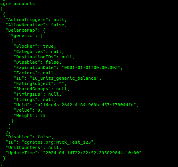
Alright, now let’s take a quick sidebar, and check in with cgr-console in a different tab, what do we think is going to show as our balance?
Well, if we run the accounts command from within cgr-console we can see our account which had a balance of 10 before, now has a balance of 9, as we’ve deducted 1 from the balance by inputting it as our usage:
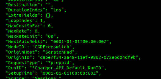
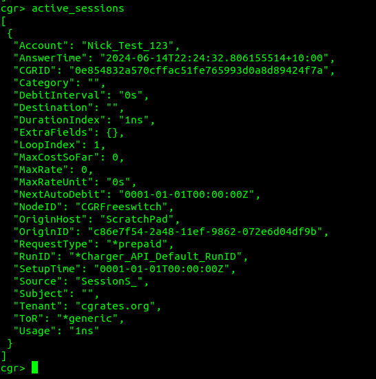
And if we run the active_sessions command in the same console, we see the active sessions, where we can see where that one unit of balance went.
A few things to call out here:
The DebitInterval is how often this balance will be deducted, for our test scenario we’ve turned off automatic debiting, but Agents like FreeSWITCH and Kamailio leave this on and automatically tick off time as it passes (Obliviously this doesn’t work for data, so we’d leave it off)
The LoopIndex is how many UpdateSessions events the API has handled for this session (the unique session is identified by the ID / CGRID field)
SetupTime is blank because we didn’t set it in our initial UpdateSession API Call
The Usage in cgr-console is sometimes shown as nanoseconds, that’s because 1ns is equal to 1 generic unit.
So let’s go back to our Python script, go through the loop again but this time set the usage to 7.
Now if we flip back to cgr-console and check again, we’ll see, as expected that our account balance is now 2, and the active session has 8 of usage.
That’s because we started with 10, then we deducted 1, then we deducted 7, gives us 2 remaining. If we’re to run active_sessions again at cgr-console we’ll see the Usage of the session is now 8.
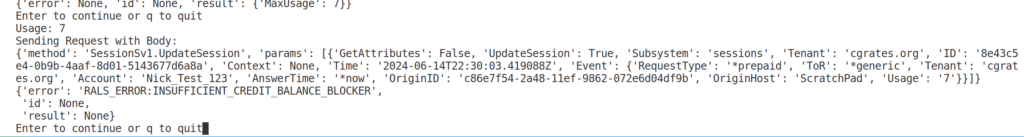
And lastly let’s try and take another 7 of balance, knowing we’ve only got 2 units left.
No dice; 7 is greater than 2 of course, so CGrateS stops us there by rejecting the request with RALS_ERROR:INSUFFICNET_CREDIT_BALANCE_BLOCKER – SessionS has done it’s job of making sure we didn’t allocate more of the credit than we were allowed and told us we have insufficient credit and that this balance is a blocker.
In this little demo we had one service drawing on the same source, but imagine if you’d fired up two copies of the script, you could have those two sources both consuming data at the same time, and this is where CGrateS shines; CGrateS can do all the heavy lifting to make sure that the resources are never over allocated, and that we’re not ending up with a negative balance.
When it comes time to terminating the session, there’s a trick to this.
Unit reservation is all about allocating resources in advance, this means we’ve generally have taken more money from the balance than we actually ended up consuming, so we have to give this back to the customer.
If we include the Usage field in the TerminateSession request, this must be the total usage for the entire session (start-to-finish), not just since the last UpdateSession API call.
For example if we allocated 30 seconds balance at the start of a call, then as that 30 seconds was consumed, we allocated another 30 seconds, and then when the call got 60 seconds in, we allocate another 30 seconds of balance. But if the call ends at a total of 70 seconds, we’ve allocated 90 seconds (3x 30 seconds), so we’d be over billing the customer. This is where we set Usage to 70 and CGrateS will refund the 20 seconds of balance we over charged them. This is because 3x 30 seconds = 90 seconds allocated, but the call only ended up using 70 seconds, so we need to refund 20 seconds of balance (90 – 70 = 20) to the Account balance.
That’s one way of doing it, but the other option is if we’ve just tracked usage since the last update, we have a 70 second call that we had allocated 3x 30 seconds Session Updates, we can set LastUsed to be 10 seconds (as we only used 10 seconds of the 30 seconds allocated in the last Update) which will also refund the 20 seconds.
In practice, you’ll probably use CGrateS Agents like the FreeSWITCH Agent, Asterisk Agent or Kamailio Agent to handle the charging in those applications. By using the premade CGrateS Agents, it handles generating the UpdateSession calls and all of this logic under the hood, but it’s super useful to know how it all works.
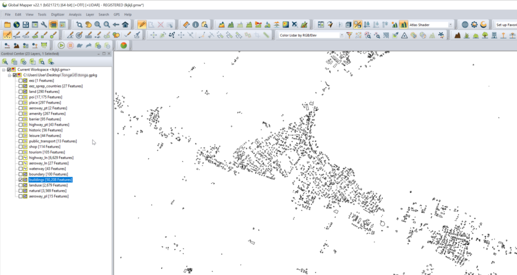
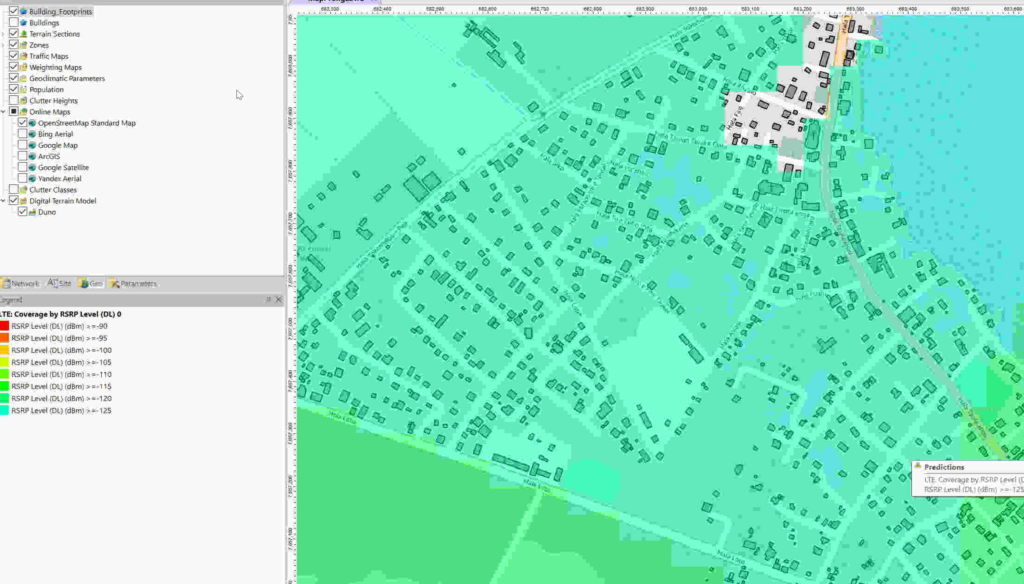
Having building footprints inside Atoll is super-duper valuable, this means you can calculate your percentage of homes / buildings covered, after all geographic coverage and population coverage are two very different things.
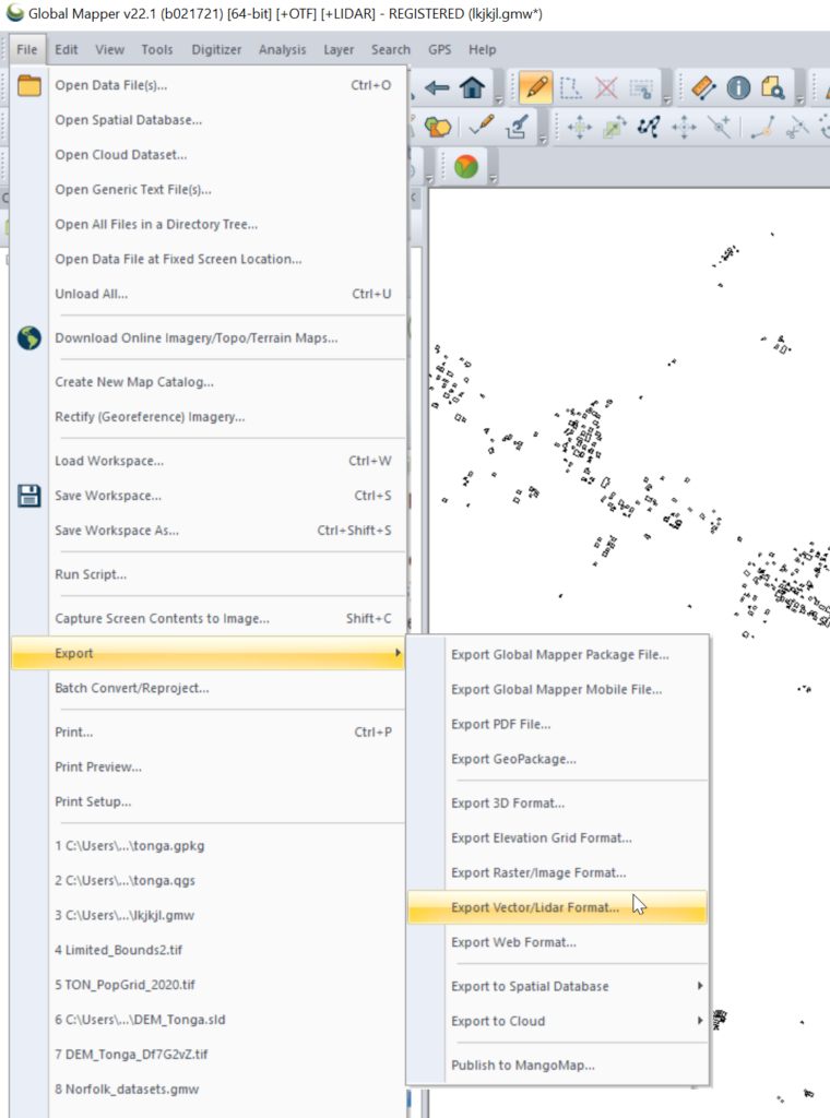
Once you’ve got the export, we’ll load the .gpkg file (or files) into GlobalMapper
Select one layer at a time that you want to export into Atoll. (This also works for roads, geographic boundaries, POIs, etc)
Export the selected layer from Export -> Export Vector / Lidar Format
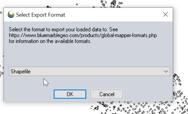
Set output type to “Shapefile”
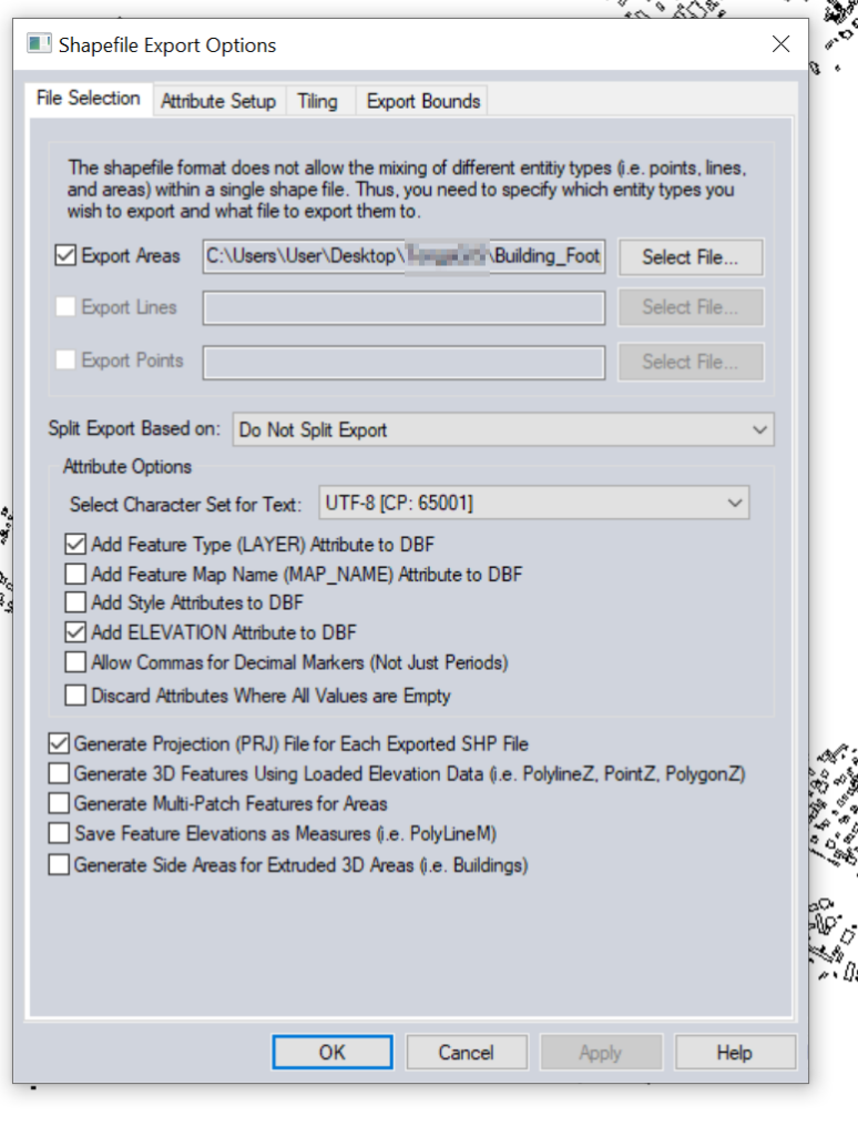
Set output filename in “Export Areas” (This will be the output file). If you want to limit the export to a given area you can do that in Export Bounds.
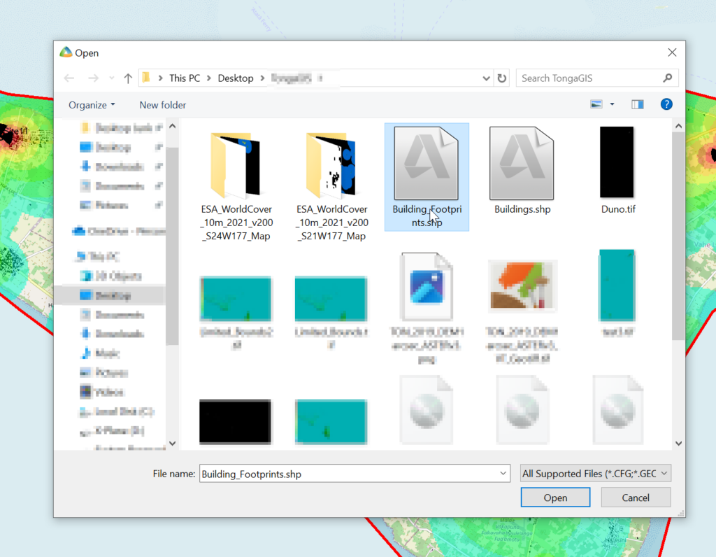
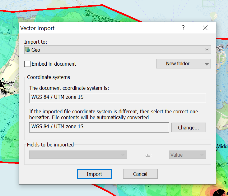
Now we can import this data into Atoll.
File -> Import
Select the exported Shapefile we just created.
Set the projection and import
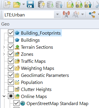
Bingo now we’ve got our building footprints,
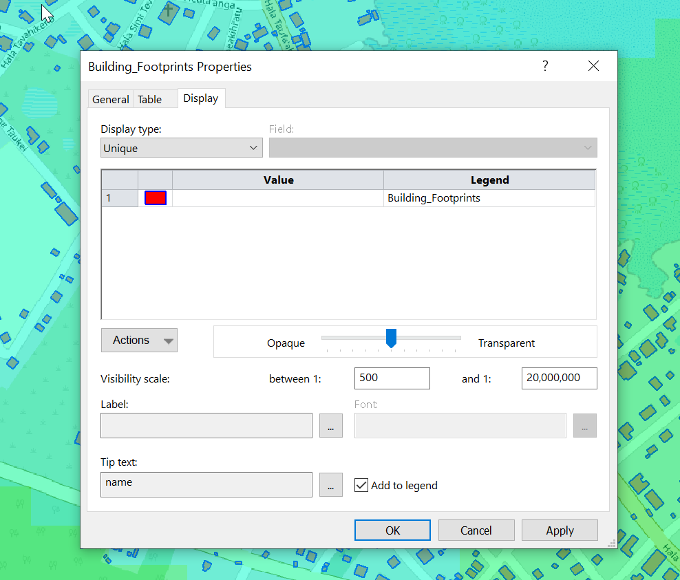
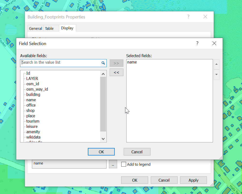
We can change the style of the layer and the labels as needed.
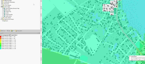
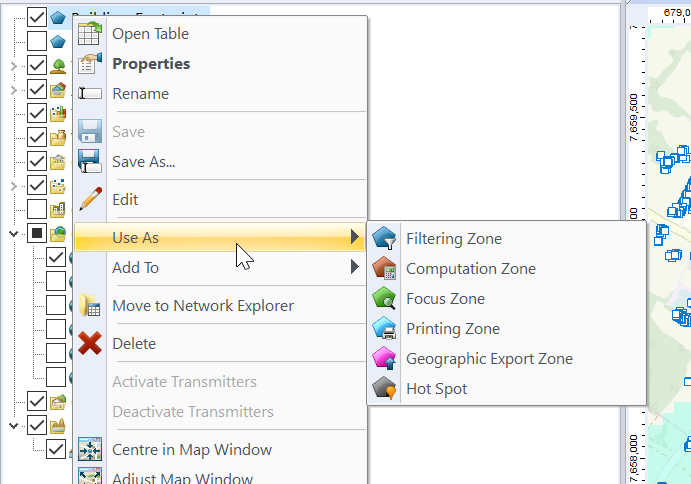
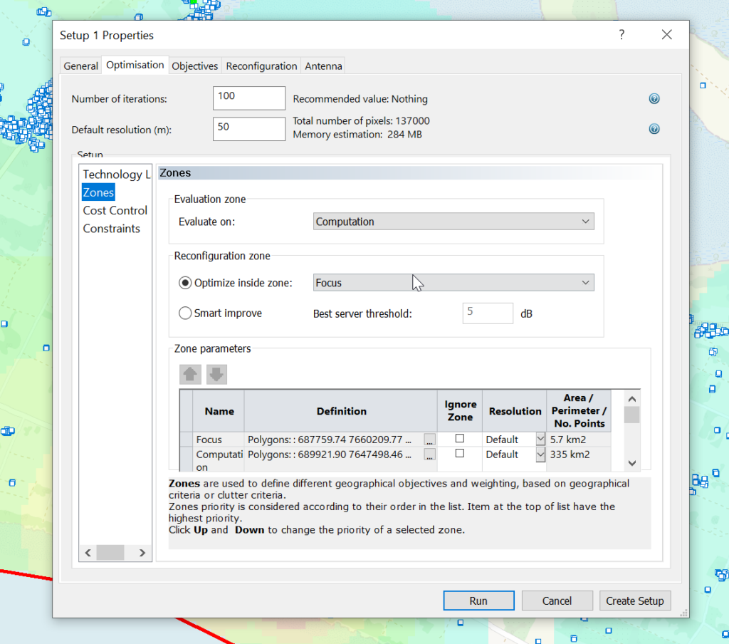
Now we can use the buildings as the Focus Zone / Compute Zone and then run reports and predictions based on those areas.
For example I can run Automatic Cell Planning with the building layers as the Focus zones, to optimize azimuths, tilts and powers to provide coverage to where people live, not just vacant land.
Clutter data describes real world things on the planet’s surface that attenuate signals, for example trees, shrubs, buildings, bodies of water, etc, etc. There’s also different types of trees, some types of trees attenuate signals more than others, different types of buildings are the same.
Getting clutter data used to be crazy expensive, and done on a per country or even per region basis, until the European Space Agency dropped a global dataset free of charge for anyone to use, that covered the entire planet in a single source of data.
So we can use this inside Forsk Atoll for making our predictions.
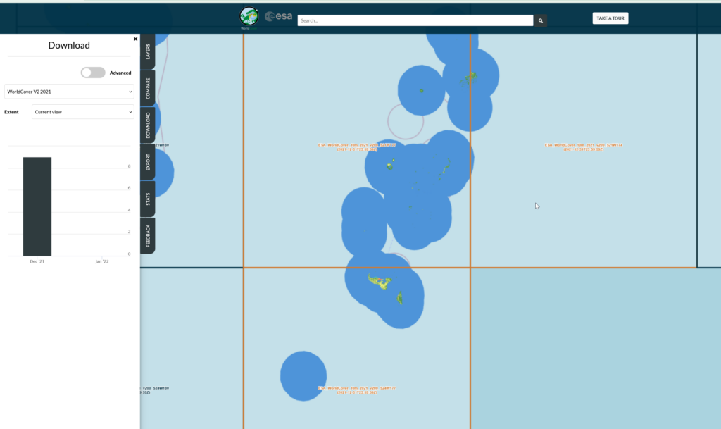
First things first we’ll need to create an account with the ESA (This is not where they take astronaut applications unfortunately, it just gives you access to the datasets).
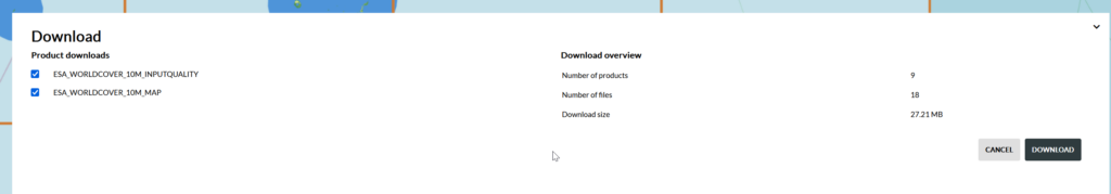
Then you can select the areas (tiles) you want to download after clicking the “Download” tab on the right.
We get a confirmation of the tiles we’re download and we’ll get a ZIP file containing the data.
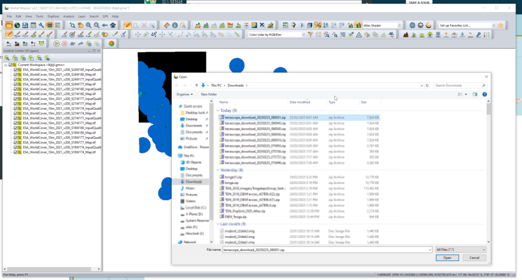
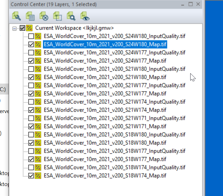
We can load the whole ZIP file (Without needing to extract anything) into GlobalMapper which loads all the layers.
I found the _Map.tif files the highest resolution, so I’m only exporting these.
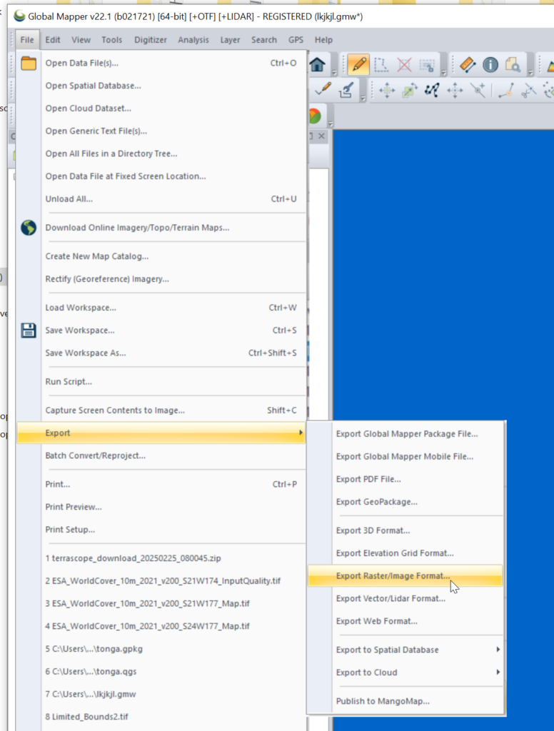
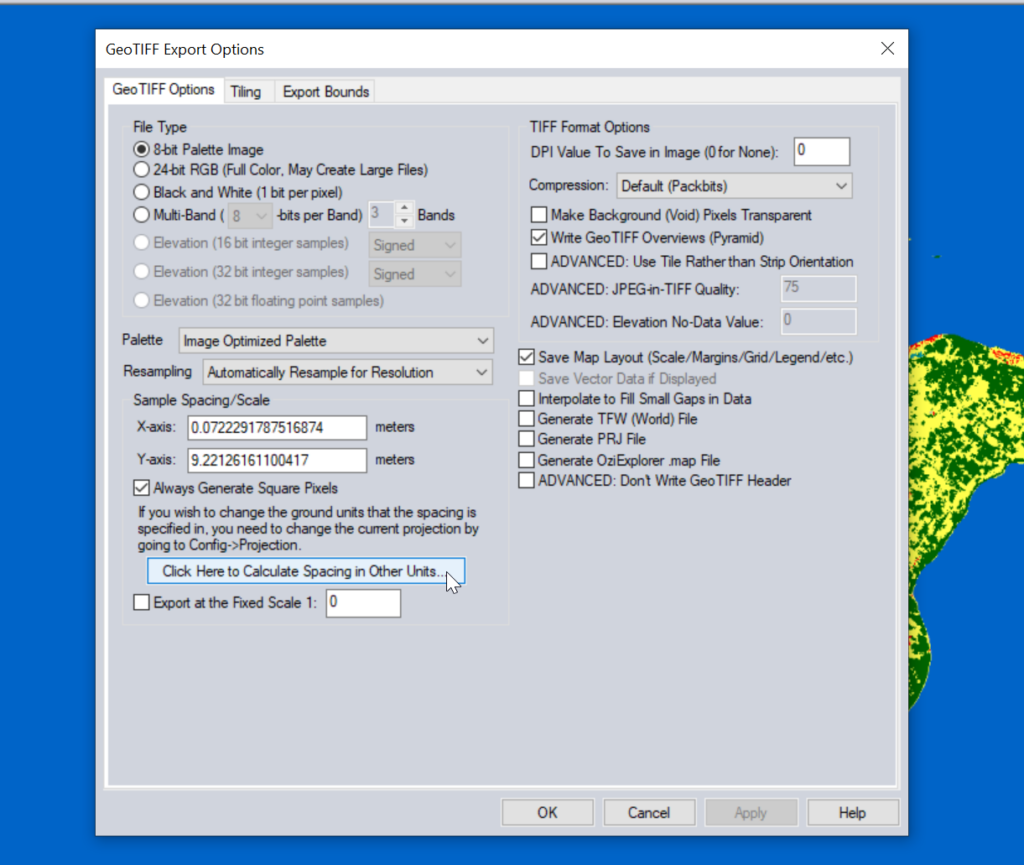
Then we need to export the data to GeoTiff for use in Atoll (The specific GeoTiff format ESA produces them in is not compatible with Atoll hence the need to convert), so we export the layers as Raster / Image format.
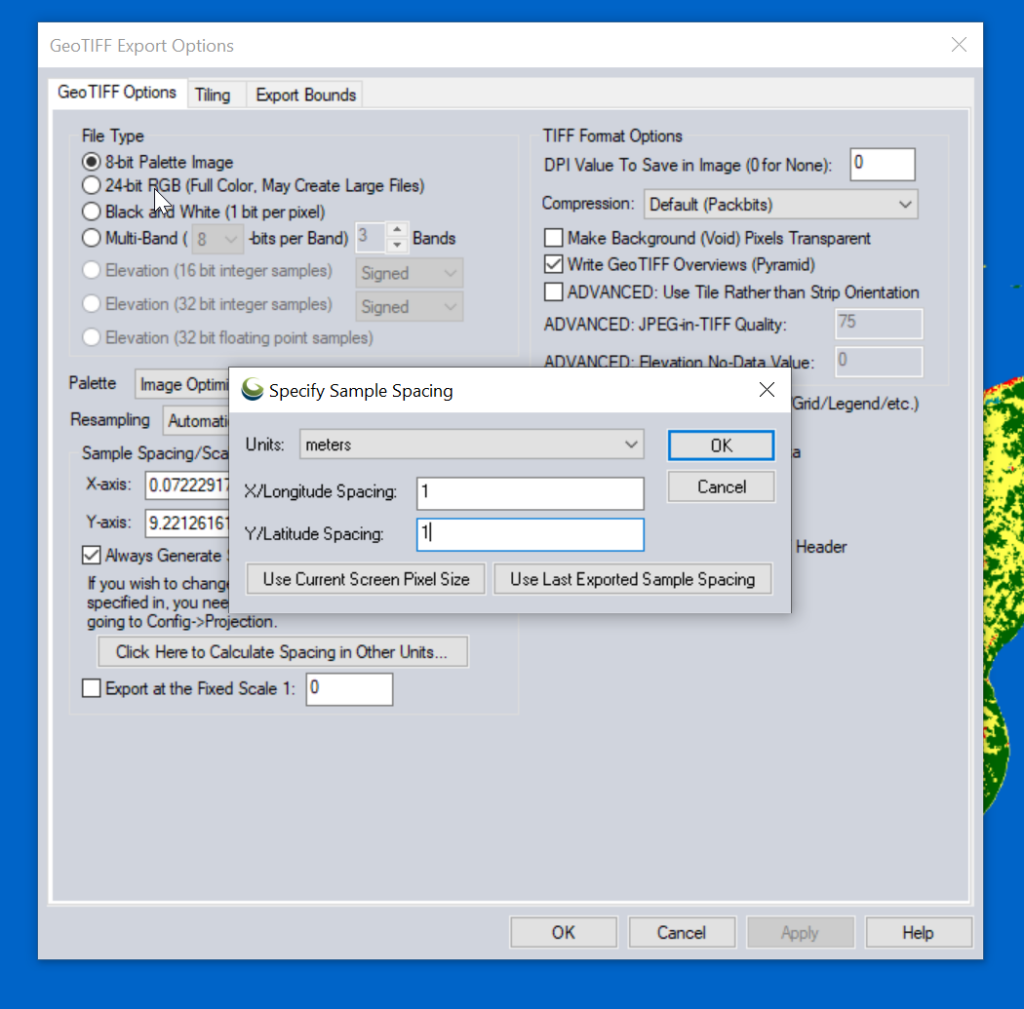
Atoll requires square pixels, and we need them in meters, so we select “Calculate Spacing in Other Units”.
Then set the spacing to meters (I use 1m to match everything else, but the data is actually only 10m accurate, so you could set this to 10m).
You probably want to set the Export Bounds to just the areas you’re interested in, otherwise the data gets really big, really quickly and takes forever to crunch.
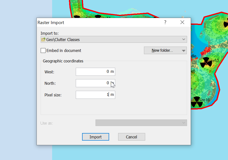
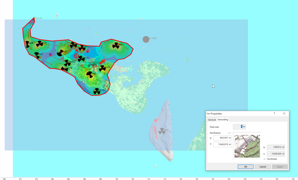
Now for the fancy part, we need to import it into Atoll.
When we import the data we import it as Raster data (Clutter Classes) with a pixel size of 1m.
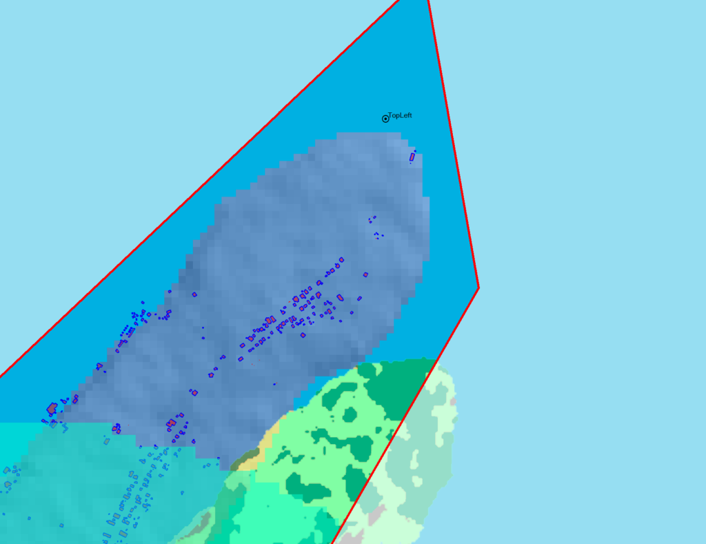
Alas when we exported the data we’ve lost the positioning information, so while we’ve got the clutter data, it’s just there somewhere on the planet, which with the planet being the size it is, is probably not where you need it.
So I cheat, I start put putting the West and North values to match the values from a Cell Site I’ve already got on the map (I put one in the top left and bottom right corners of the map) and use that as the initial value.
Then – and stick with me, this is very technical – I mess with the values until the maps line up into the correct position. Increase X, decrease Y, dialing it it in until the clutter map lines up with the other maps I’ve got.
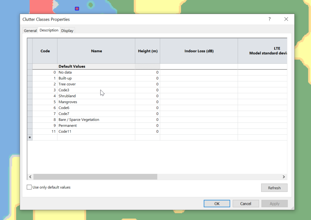
Right, now we’ve got the data but we don’t have any values.
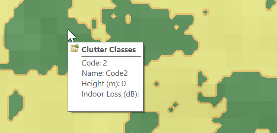
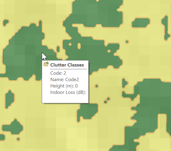
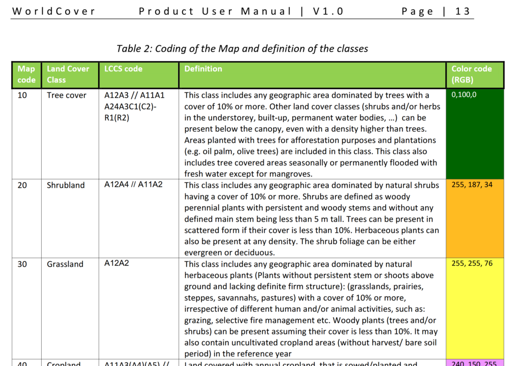
Each color represents a clutter class, but we haven’t set any actual height or losses for that material.
Alas the Map Code does not match with the table in the manual, but the colours do, here’s what mine map to:
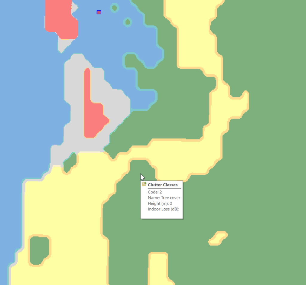
Which means when hovering over a layer of clutter I can see the type:
Next we need to populate the heights, indoor and outdoor losses for that given clutter. This is a little more tricky as it’s going to vary geography to geography, but there’s indicative loss numbers available online pretty easily.
Once you’ve got that plugged in you can run your predictions and off you go!
Another post in the “vendors thought Java would last forever but the web would just a fad” series, this one on getting Nokia BTS Site Manager (which is used to administer the pre-Airscale Nokia base stations) running on a modern Linux distro.
For starters we get the installers (you’ll need to get these from Nokia), and install openjdk-8-jre using whichever package manager your distro supports.
Once that’s installed, then extract the installer folder (Like BTS Site Manager FL18_BTSSM_0000_000434_000000-20250323T000206Z-001.zip).
Inside the extracted folder we’ve got a path like:
BTS Site Manager FL18_BTSSM_0000_000434_000000-20250323T000206Z-001/BTS Site Manager FL18_BTSSM_0000_000434_000000/C_Element/SE_UICA/Setup
The Setup folder contains a bunch of binaries.
We make these executable:
chmod +x BTSSiteEM-FL18-0000_000434_000000*
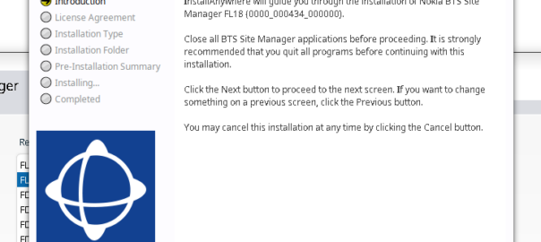
Then run the binary:
sudo ./BTSSiteEM-FL18-0000_000434_000000_x64.bin
By default it installs to /opt/Nokia/Managers/BTS\ Site/BTS\ Site\ Manager
And we’re done. Your OS may or may not have built a link to the app in your “start menu” / launcher.
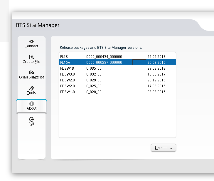
You can use one BTS manager to manage several different versions of software, but you need the definitions for those software loaded.
If you want to load the Releases for other versions (Like other FLF or FL releases) the simplest way is just to install the BTS site manager for those versions and just use the latest, then you’ll get the table of installed versions in the “About” section that you can administer.
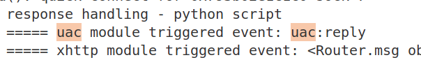
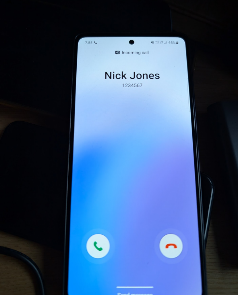
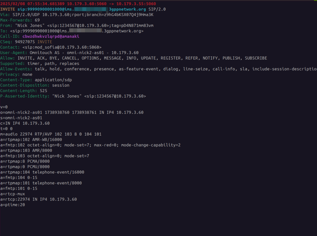
SIP has got a multitude of ways of showing Caller ID, PAI, R-PAI, From, even Contact, but the other day I got a tip (Thanks John!) that you can set a name as the Caller ID in the “Username field “display name” part of the P-Asserted-Identity for the leg from the TAS to the UE, and it’ll show up on the phone, and they’re right.
One thing that it doesn’t do is show the name in the call history, and if you go to “Add as Contact” it still makes you enter the name, clearly that’s not linked in, but it’s a kinda neat feature.
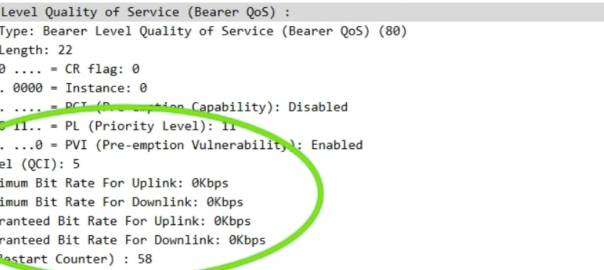
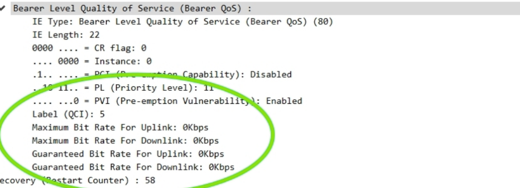
The other day I had a query about a roaming network that was sending Bearer Level QoS parameters in the Create Session Request to 0Kbps, up and down rather than populating the MBR values.
I knew for Guaranteed Bit Rate bearers that this was of course set, but for non GBR bearers (QCI 5 to 9) I figured this would be set the to MBR, but that’s not the case.
So what gives?
Well, according to TS 29.274:
For non-GBR bearers, both the UL/DL MBR and GBR should be set to zero.
So there you have it, if it’s not a QCI 1-4 bearer then these values are always 0.
Concrete, steel and labor are some of the biggest costs in building a cell site, and yet all the focus on cost savings for cell sites seems to focus on the RAN, but the actual RAN equipment isn’t all that much when you put it into context.
I think this is mostly because there aren’t folks at MWC promoting concrete each year.
But while I can’t provide any fancy tricks to make towers stronger or need less concrete for foundations, there’s some potential low-hanging fruit in terms of installation of sites that could save time (and therefor cost) during network refreshes.
I don’t think many folks managing the RAN roll-outs for MNOs have actually spent a week with a tower crew rolling this stuff out. It’s hard work but a lot of it could be done more efficiently if those writing the MOPs and deciding on the processes had more experience in the field.
Disclaimer: I’m primarily a core networks person, this is the job done from a comfy chair. This is just some observations from the bits of work I’ve done in the field building RAN.
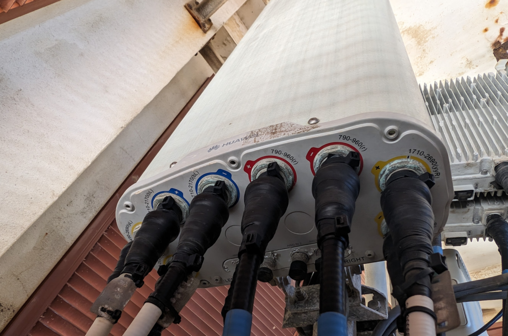
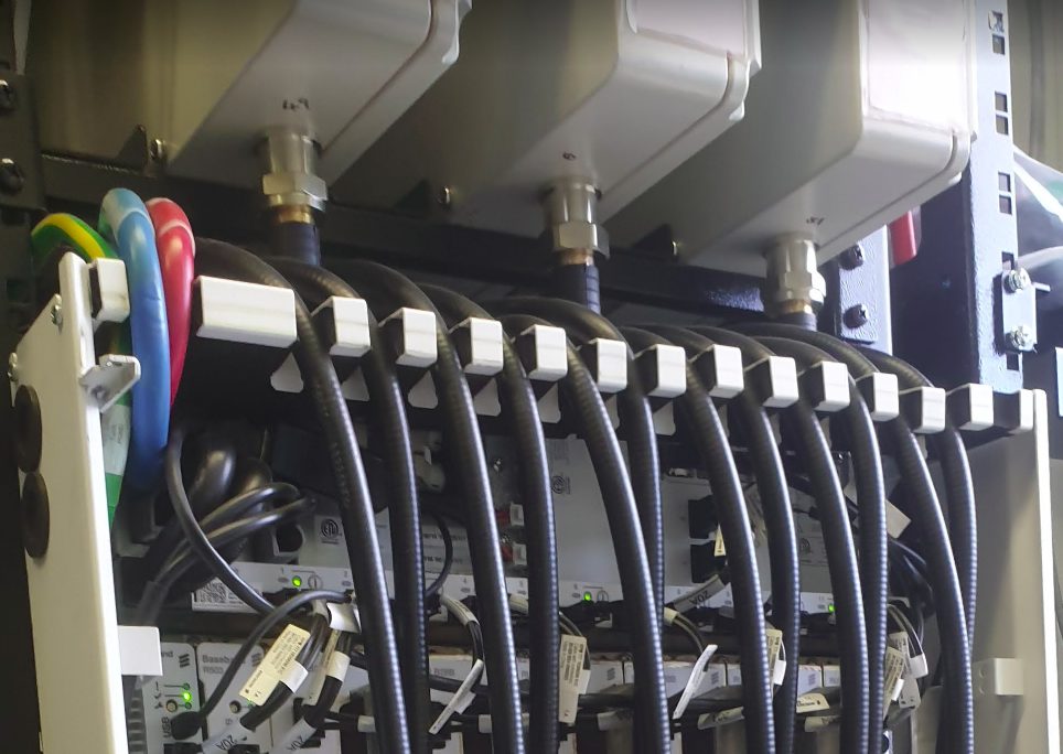
Standardize Power Connectors
Currently radio units from the biggest RAN vendors (Ericsson, Nokia, Huawei, ZTE & Samsung) each use different DC power connectors.
This means if you’re swapping from one of these vendors to another as part of a refresh, you need new power connectors.
If you’re lucky you’re able to reuse the existing DC power cables on the tower, but that means you’re up on a tower trying to re-terminate a cable which is a fiddly job to do on the ground, and far worse in the air. Or if you’re unlucky you don’t have enough spare distance on the DC cables to do the job, then you’re hauling new DC cables up a tower (and using more cables too).
While Huawei and ZTE have adopted for push connectors with the raw cables behind a little waterproof door.
If we could just settle on one approach (either is fine) this could save hours of install time on each cell site, extrapolate that across thousands of cell sites for each network, and this is a potentially large saving.
Standardize Fiber Cables
The same goes for waterproofing fibre, Ericsson has a boot kit that gets assembled inline over the connectors, Nokia has this too, as well as a rubber slide over cover boot on pre-term cables.
Again, the cost is fairly minimal, but the time to swap is not. If we could standardize a break out box format on the top of the tower and a LC waterproofing standard, we could save significant time during installs, and as long as you over-provision the breakout (The cost difference between a 6 core fiber vs a 48 core fibre is a few dollars), you can save significant time having to rerun cables.
Yes, we’ve all got horror stories about someone over-bending fiber, and if you reused fibre between hardware refresh cycles, but modern fiber is crazy tough so the chances of damaging the reused fiber is pretty slim, and spare pairs are always a good thing.
Preterm DC Cables
Every cell site install features some poor person squatting on the floor (if they’re savvy they’ve got a camping stool or gardening kneeling mat) with a “gut buster” crimping tool swaging on connectors for the DC lugs.
If we just used the same lugs / connectors for all the DC kit inside the cell sites, we could have premade DC cables in various lengths (like everyone does with Ethernet cables now), rather than making each and every cable off a spool (even if it is a good ab workout).
I dunno, I’m just some Core network person who looks at how long all this takes and wonders if there’s a way it could be done better, am I crazy?
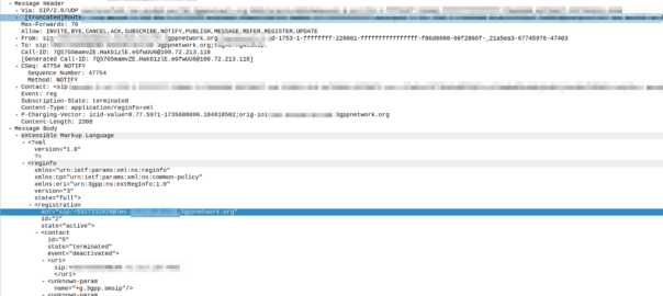
Nope – it doesn’t do anything useful. So why is it there?
The SUBSCRIBE method in SIP allows a SIP UAC to subscribe to events, and then get NOTIFY messages when that event happens.
In a plain SIP scenario (RFC 3261), we can imagine an IP Phone and a PBX scenario. I might have “Busy Lamp Field” aka BLF buttons on the screen of my phone, that change colour when the people I call often are themselves on calls or on DND, so I know not to transfer calls to them – This is often called the “presence” scenario as it allows us to monitor the presence of another user.
At a SIP level, this is done by sending a SUBSCRIBE to the PBX with the information about what I’m interested in being told about (State changes for specific users) and then the PBX will send NOTIFY messages when the state changes.
But in IMS you’ll see SUBSCRIBE messages every time the subscriber registers, so what are they subscribing for?
Well, you’re just subscribing to your own registration status, but your phone knows your own registration status, because it’s, well, the registration status of the phone.
So what does it achieve? Nothing.
The idea was in a fixed-mobile-convergence scenario (keeping in mind that’s one of the key goals from the 2008 IMS spec) you could have the BLF / presence functionality for fixed subscribers, but this rareley happens.
For the past few years we’ve just been sending a 200 OK to SUBSCRIBE messages to the IMS, with a super long expiry, just to avoid wasting clock cycles.
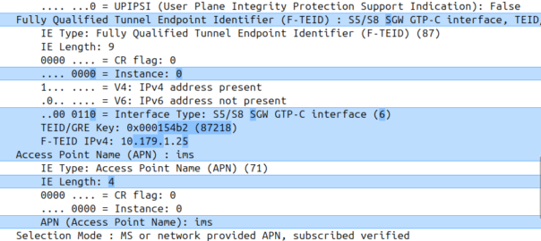
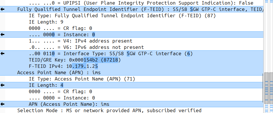
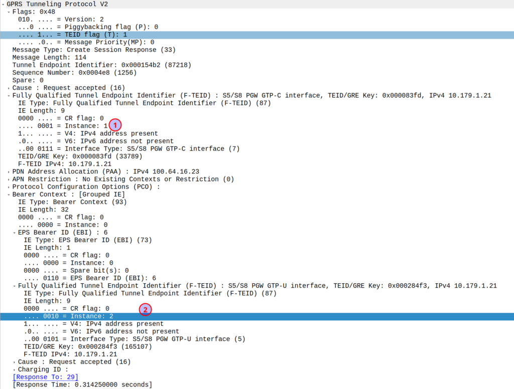
I was diffing two PCAPs the other day trying to work out what’s up, and noticed the Instance ID on a GTPv2 IE was different between the working and failing examples.
If more than one grouped information elements of the same type, but for a different purpose are sent with a message,
these IEs shall have different Instance values.
So if we’ve got two IEs of the same IE type (As we often do; F-TEIDs with IE Type 87 may have multiple instances in the same message each with different F-TEID interface types), then we differentiate between them by Instance ID.
The only exception to this rule is where we’ve got the same data, so if you’ve got one IE with the exact same values and purpose that exists twice inside the message.
Last year we deployed some Hughes HL1120W OneWeb terminals in one of the remote cellular networks we support.
Unfortunately it was failing to meet our expectations in terms of performance and reliability – We were seeing multiple dropouts every few hours, for between 30 seconds and ~3 minutes at a time, and while our reseller was great, we weren’t really getting anywhere with Eutelsat in terms of understanding why it wasn’t working.
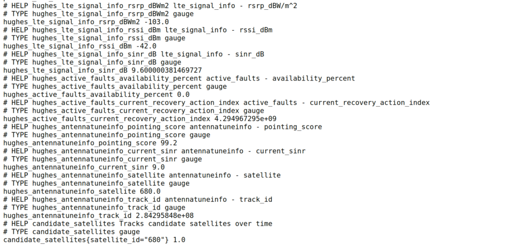
Luckily for us, Hughes (who manufacture the OneWeb terminals) have an unprotected API (*facepalm*) from which we can scrape all the information about what the terminal sees.
As that data is in an API we have to query, I knocked up a quick Python script to poll the API and convert the data from the API into Prometheus data so we could put it into Grafana and visualise what’s going on with the terminals and the constellation.
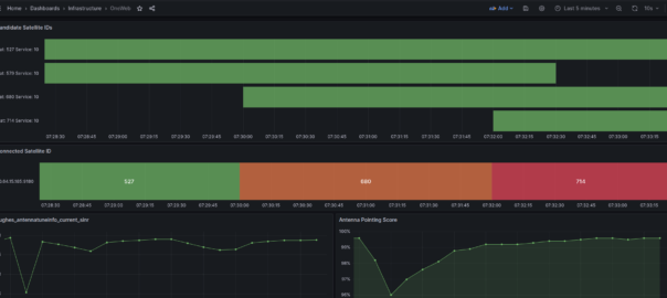
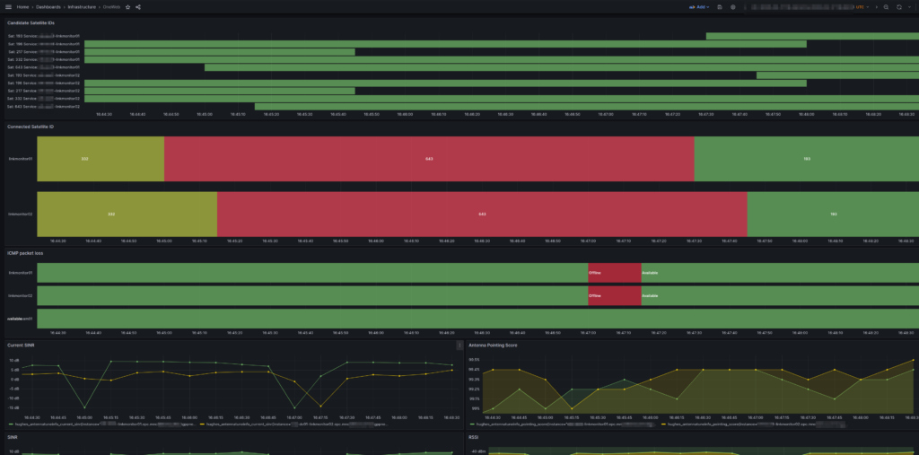
After getting all this into Grafana and combining it with the ICMP Blackbox exporter (we configured Blackbox to send HTTP requests and ICMP pings out of each of the different satellite terminals we had (a mix of OneWeb and others)) we could see a pattern emerging where certain “birds” (satellites) that passed overhead would come with packet loss and dropouts.
It was the same satellites each time that led to the drops, which allowed us to pinpoint to say when we see this satellite coming over the horizon, we know there’s going to be some packet loss.
In the end Eutelsat acknowledged they had two faulty satellites in the orbit we are using, hence seeing the dropouts, and they are currently working on resolving this (but that actually does require rockets, so we’re left without a usable service for the time being) but it was a fun problem to diagnose and a good chance to learn more about space.
Packet loss on the two OneWeb terminals (Not seen on other constellation) correlated with a given satellite pass
The repo has instructions for use and the Grafana templates we used.
At one point I started playing with the OneWeb Ephemeris data so I could calculate the azimuth and elevation of each of the birds from our relative position, and work out distances and angles from the terminal. The maths was kinda fun, but oddly the datetimes in the OneWeb ephemeris data set seems to be about 10 years and 10 days behind the current datetime – Possibly this gives an insight into OneWeb’s two day outage at the start of the year due to their software not handling leap years.
Despite all these teething issues I’m still optimistic about OneWeb, Kupler and Qianfan (Thousand Sails) opening up the LEO market and covering more people in more places.
Update: Thanks to Scott via email who sent this: One note, there’s a difference between GPS time and Unix time of about 10 years 5 days. This is due to a) the Unix epoch starting 1970-01-01 and the gps epoch starting 1980-01-05 and b) gps time is not adjusted for leap seconds, and ends up being offset by an integer number of seconds.