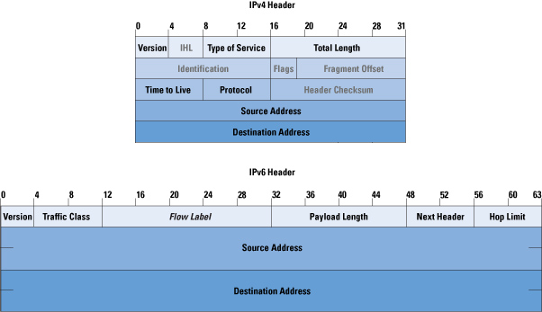
SGs-AP which is used for CSFB & SMS doesn’t span network borders (you can’t roam with SGs-AP), and with SMSoIP out of the question, that gave us the option of MAP or Diameter, so we picked Diameter.
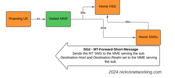
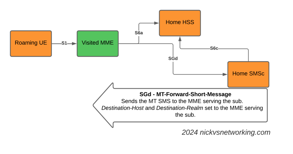
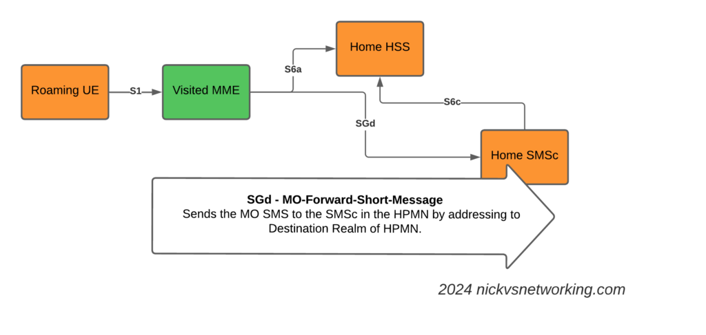
This introduces the S6c and SGd Diameter interfaces, in the diagrams below Orange is the Home Network (HPMN) and the Green is the Visited Network (VPMN).
The S6c interface is used between the SMSc and the HSS, in order to retrieve the routing information. This like the SRI-for-SM in MAP.
The SGd interface is used between the MME serving the UE and the SMSc, and is used for actual delivery of the MO/MT messages.
I haven’t shown the Diameter Routing Agents in these diagrams, but in reality there would be a DRA on the VPLMN and a DRA on the HPMN, and probably a DRA in the IPX between them too.
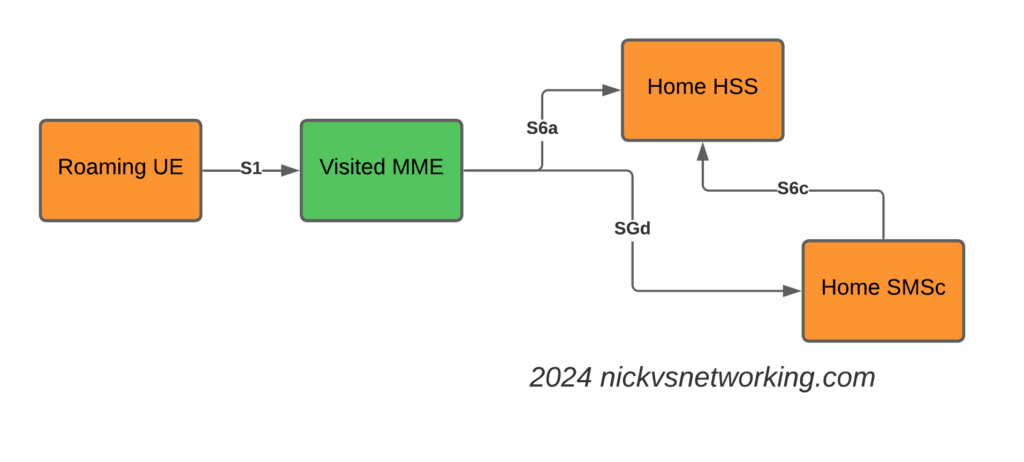
The Attach
The attach looks like a regular roaming attach, the MME in the Visited PMN sends an Update Location Request to the HSS, so the HSS knows the MME that is serving the subscriber.
S6a Update Location Request to indicate the MME serving the Subscriber
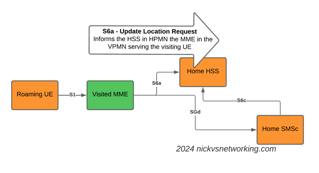
The Mobile Terminated SMS Flow
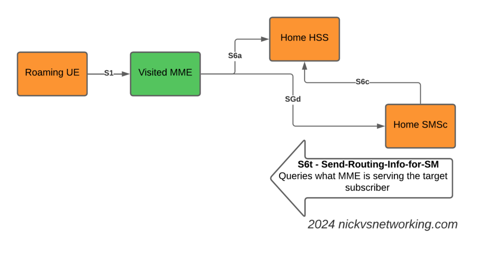
Now we introduce the S6c interface and the SGd interfaces.
When the Home SMSc has a message to send to the subscriber (Mobile Terminated SMS) it runs a the Send-Routing-Info-for-SM-Request (SRR) dialog to the HSS.
The Send-Routing-Info-for-SM-Answer (SRA) back from the HSS contains the info on the MME Diameter Host name and Diameter Realm serving the subscriber.
S6t – Send-Routing-Info-for-SM request to get the MME serving the subscriber
With this info, we can now craft a Diameter Request that will get sent to the MME serving the subscriber, containing the SMS PDU to send to the UE.
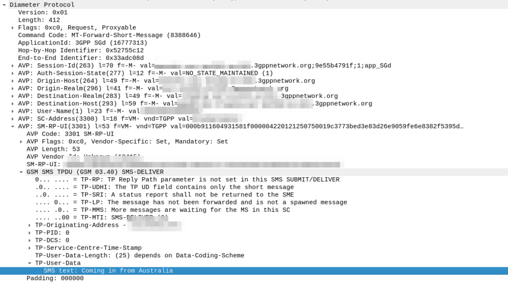
SGd MT-Forward-Short-Message to deliver Mobile Terminated SMS to the serving MME
We make sure it’s sent to the correct MME by setting the Destination-Host and Destination-Realm in the Diameter request.
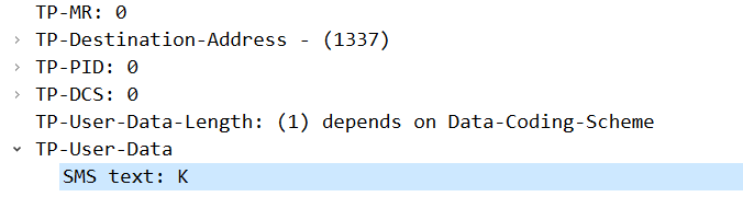
Here’s how the request looks from the SMSc towards our DRA:
As you can see the Destination Realm and Destination-Host is set, as is the User-Name set to the IMSI of the UE we want to send the message to.
And down the bottom you can see the SMS-TPDU, the same as it’s been all the way back since GSM days.
The Mobile Originated SMS Flow
The Mobile Originated flow is even simpler, because we don’t need to look up where to route it to.
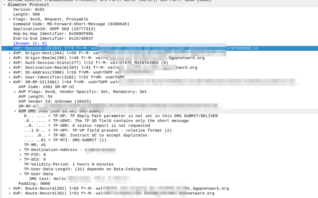
The MME receives the MO SMS from the UE, and shoves it into a Diameter message with Application ID set to SGd and Destination-Realm set to the HPMN Realm.
When the message reaches the DRA in the HPMN it forwards the request to an SMSc and then the Home SMSc has the message ready to roll.
To make more Money (This post, congratulations, you’re reading it!)
Because they have to (Regulatory compliance, insurance, taxes, etc) – That’s the next post
So let’s look at SA in this context.
5G-SA can drive new revenue streams
We (as an industry) suck at this.
Last year on the Telecoms.com podcast, Scott Bicheno made the point that if operators took all the money they’d gambled (and lost) on trying to play in the sports rights, involvement in media companies, building their own streaming apps, attempts at bundling other utilities, digital identity, etc, and just left the cash in the bank and just operated the network, they’d be better off.
Uber, Spotify, “OTTs”, etc, utilize MNOs to enable their services, but operators don’t see this extra revenue. While some operators may talk of “fair share” the truth is, these companies add value to our product (connectivity) which as an industry, we’ve failed to add ourselves.
If the Metaverse does turn out to be a cash cow, it is unlikely the telecommunications industry will be the ones milking it.
Claim: Customers are willing to pay more for 5G-SA
This myth seems to be fairly persistent, but with minimal data to support this claim.
While BSS vendors talk about “5G Monetization”, the truth is, people use their MNO to provide them connectivity. If the coverage is adequate, and the speed enough to do what they need to do, few would be willing to pay any additional cash each month to see higher numbers on a speedtest result (enabled by 5G-NSA) and even fewer would pay extra cash for, well, whatever those features only enabled by 5G-Standalone are?
With most consumers now also holding onto their mobile devices for longer periods of time, and with interest rates reining in consumer spending across the board, we are seeing the rise of a more cost conscious consumer than ever before. If we want to see higher ARPUs, we need to give the consumer a compelling reason to care and spend their cash, beyond a speed test result.
We talk a little about APIs lower down in the post.
Claim: Users want Ultra-Low Latency / High Reliability Comms that only 5G-SA delivers
Wanting to offer a product to the market, is not the same as the market wanting a product to consume.
Telecom operators want customers to want these services, but customer take up rates tell a different story. For a product like this to be viable, it must have a wide enough addressable market to justify the investment.
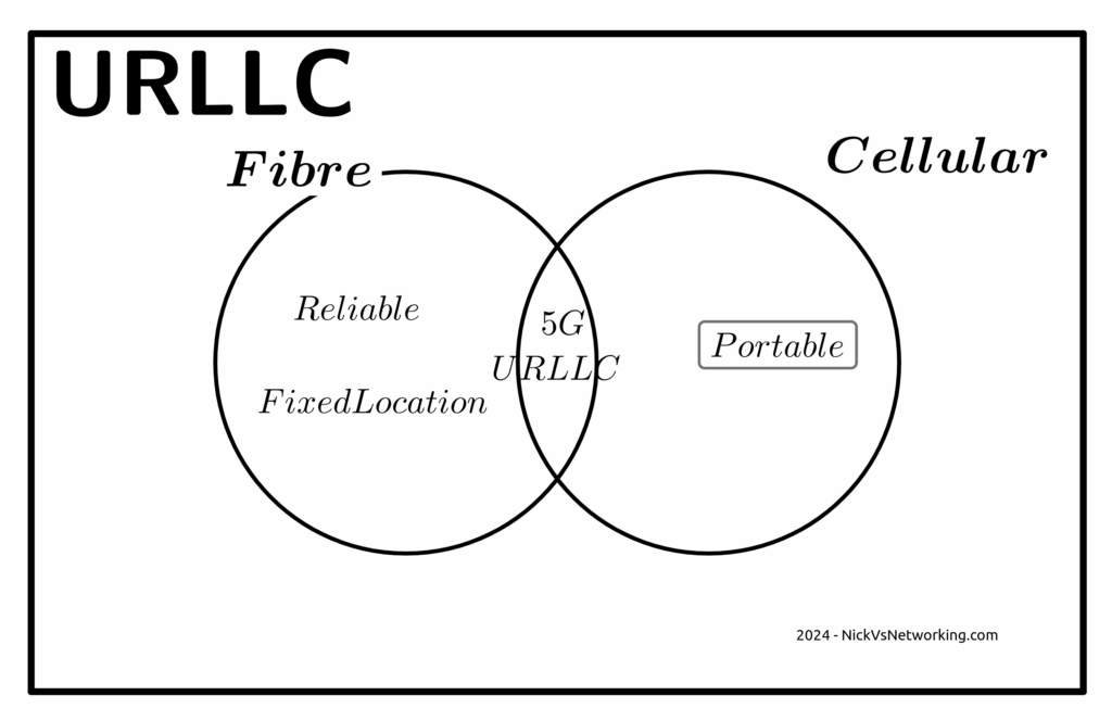
Reliability
The URLCC standards focus on preventing packet loss, but the world has moved on from needing zero packet loss.
The telecom industry has a habit of deciding what customers want without actually listening. When a customer talks about wanting “reliable” comms, they aren’t saying they want zero packet loss, but rather fewer dropouts or service flaps. For us to give the customer what they are actually asking for involves us expanding RAN footprint and adding transmission diversity, not 5G-SA.
The “protocols of the internet” (TCP/IP) have been around for more than 50 years now.
These protocols have always flowed over transport links with varied reliability and levels of packet loss.
Thanks to these error correction and retransmission techniques built into these protocols, a lost packet will not interrupt the stream. If your nuclear command and control network were carried over TCP/IP over the public internet (please don’t do this), a missing packet won’t lead to worldwide annihilation, but rather the sender will see the receiver never acknowledged the receipt of the packet at the other end, and resend it, end of.
If you walk into a hospital today, you’ll find patient monitoring devices, tracking the vital signs for patients and alerting hospital staff if a patient’s vital signs change. It is hard to think of more important services for reliability than this.
And yet they use WiFi, and have done for a long time, if a packet is lost on WiFi (as happens regularly) it’s just retransmitted and the end user never knows.
Autonomous cars are unlikely to ever rely on a 5G connection to operate, for the simple reason that coverage will never be 100%. If your car stops because you’re in a not-spot, you won’t be a happy customer. While plenty of cars have cellular modems in them, that are used to upload telemetry data back to the manufacturer, but not to drive the car.
One example of wireless controlled vehicles in the wild is autonomous haul trucks in mines. Historically, these have used WiFi for their comms. Mine sites are often a good fit for Private LTE, but there’s nothing inherent in the 5G Standalone standard that means it’s the only tool for the job here.
Slicing
Slicing is available in LTE (4G), with an architecture designed to allow access to others. It failed to gain traction, but is in networks today.
The RAN a piece of the latency puzzle here, but it is just one piece of the puzzle.
If we look at the flow a packet takes from the user’s device to the server they want to talk to we’ve got:
Time it takes the UE to craft the packet
Time it takes for the packet to be transmitted over the air to the base station
Time it takes for the packet to get through the RAN transmission network to the core
Time it takes the packet to traverse the packet core
Time it takes for the packet to get out to transit/peering
Time it takes to get the packet from the edge of the operators network to the edge of the network hosting the server
Time it takes the packet through the network the server is on
Time it takes the server to process the request
The “low latency” bit of the 5G puzzle only involves the two elements in bold.
If you’ve got to get from point A to point B along a series of roads, and the speed limit on two of the roads you traverse (short sections already) is increased. The overall travel time is not drastically reduced.
I’m lucky, I have access to a well kitted out lab which allows me to put all of these latency figures to the test and provide side by side metrics. If this is of interest to anyone, let me know. Otherwise in the meantime you’ll just have to accept some conjecture and opinion.
You could rebut this talking about Edge Compute, and having the datacenter at the base of the tower, but for a number of fairly well documented reasons, I think this is unlikely to attract widespread deployment in established carrier networks, and Intel’s recent yearly earning specifically called this out.
Claim: Customers want APIs and these needs 5G SA
Companies like Twilio have made it easy to interact with the carrier network via their APIs, but yet again, it’s these companies producing the additional value on a service operated by the MNOs.
My coffee machine does not have an API, and I’m OK with this because I don’t have a want or need to interact with it programatically.
By far, the most common APIs used by businesses involving telco markets are APIs to enable sending an SMS to a user.
These have been around for a long time, and the A2P market is pretty well established, and the good news is, operators already get a chunk of this pie, by charging for the SMS.
Imagine a company that makes medical booking software. They’re a tech company, so they want their stack to work anywhere in the world, and they want to be able to send reminder SMS to end users.
They could get an account manager with each of the telcos in each of the markets they work in, onboard and integrate the arcane complexities of each operators wholesale SMS system, or they could use Twilio or a similar service, which gives them global reach.
Often the cost of services like Twilio are cheaper than working directly with the carriers in each market, and even if it is marginally more expensive, the cost savings by not having to deal with dozens of carriers or integrate into dozens of systems, far outweighs this.
While it’s a great idea, in the context of 5G Standalone and APIs, it’s worth noting that none of the use cases in OpenGateway require 5G Standalone (Except possibly Edge discovery, but it is debatable).
Critically, from a developer experience perspective:
I can sign up to services like Twilio without a credit card, and start using the service right away, with examples in my programming language of choice, the developer user experience is fantastic.
Jump on the OpenGateway website today and see if you can even find a way to sign up to use the service?
Claim: Fixed Wireless works best with 5G-SA
Of all the touted use cases and applications for 5G, Fixed Wireless (FWA) has been the most successful.
The great thing about FWA on Cellular networks is you can use the same infrastructure you use for your mobile customers, and then sell excess capacity in the network to deliver Fixed Wireless Access services, better utilizing an asset (great!).
But again, this does not require Standalone 5G. If you deploy your FWA network using 5G SA, then you won’t be able to sweat that same asset for both mobile subscribers and FWA subscribers.
Today at least, very few handsets short of this generation of flagship phones, supports 5G SA. Even the phones sold as supporting 5G over the past few years, are almost all only supporting 5G-NSA, so if you rolled out your FWA network as Standalone, you can’t better utilize the asset by sharing with your existing LTE/5G-NSA customers.
Claim: The Killer App is coming for 5G and it needs 5G SA
This space is reserved for the killer app that requires 5G Standalone.
Whenever that comes?
Anyone?
I’m not paying to build a marina berth for my mega yacht, mostly because I don’t have one. Ditto this.
Could you explain to everyone on an investor call that you’re investing in something where the vessel of the payoff isn’t even known to exist? Telecom is “blue chip”, hardly speculative.
The Future for Revenue Growth?
Maybe there isn’t one.
I know it’s an unthinkable thought for a lot of operators, but let’s look at it rationally; in the developed world, everyone who wants a mobile service already has one.
This leaves operators with two options; gaining market share from their competitors and selling more/higher priced services to existing customers.
You don’t steal away customers from other operators by offering a higher priced product, and with reduced consumer spending people aren’t queuing up to spend more each month.
But there is a silver lining, if you can’t grow revenues, you can still shrink expenditure, which in the end still gets the same result at the end of the quarter – More cash.
Simplify your operations, focus on what you do really well (mobile services), the whole 80/20 rule, get better at self service, all that guff.
There’s no shortage of pain points for consumers telecom operators could address, to make the customer experience better, but few that include the word Slicing.
No one spends marketing dollars talking about the problems with a tech and vendors aren’t out there promoting sweating existing assets. But understanding your options as an operator is more important now than ever before.
Sidebar; This post got really long, so I’m splitting it into 3…
We’re often asked to help define a a 5G strategy for operators; while every case is different, there’s a lot of vendors pushing MNOs to move towards 5G standalone or 5G-SA.
I’m always a fan of playing “devil’s advocate“, and with so many articles and press releases singing the praises of standalone 5G/5G-SA, so as a counter in this post, I’ll be making the case against the narratives presented to operators by vendors that the “right” way to do 5G is to introduce 5G Standalone, that they should all be “upgrading” to Standalone 5G.
With Mobile World Congress around the corner, now seems like a good time to put forward the argument against introducing 5G Standalone, rebutting some common claims about 5G Standalone operators will be told. We’ll counterpoint these arguments and I’ll put forward the case for not jumping onto the 5G-SA bandwagon – just yet.
On a personal note, I do like 5G SA, it has some real advantages and some cool features, which are well documented, including on this blog. I’m not looking to beat up on any vendors, marketing hype or events, but just to provide the “other side” of the equation that operators should consider when making decisions and may not be aware of otherwise. It’s also all opinion of course (cited where possible), but if you’re going to build your network based on a blog post (even one as good as this) you should probably reconsider your life choices.
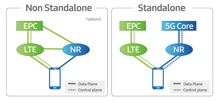
Some Arcane Detail: 5G Non-Standalone (NSA) vs Standalone (SA)
5G NSA (Non Standalone) uses LTE (4G) with an additional layer “bolted on” that uses 5G on the radio interface to provide “5G” speeds to users, while reusing the existing LTE (Evolved Packet Core) core and VoLTE for voice / SMS.
From an operator perspective there is almost no change required in the network to support NSA 5G, other than in the RAN, and almost all the 5G networks in commercial use today use 5G NSA.
5G NSA is great, it gives the user 5G speeds for users with phones that support it, with no change to the rest of the network needed.
Standalone 5G on the other hand requires an a completely new core network with all the trimmings.
While it is possible to handover / interwork with LTE/4G (Inter-RAT Handovers), this is like 3G/4G interworking, where each has a different core network. Introducing 5G standalone touches every element of the network, you need new nodes supporting the new standards for charging, policy, user plane, IMS, etc.
Scope
There’s an old adage that businesses spend money for one of three reasons:
To Save Money (Which we’ll cover in this post)
To make more Money (Covered next – Will link when published)
Because they have to (Regulatory compliance, insurance, taxes, etc)
Let’s look at 5G Standalone in each of these contexts:
5G Cost Savings – Counterpoint: The cost-benefit doesn’t stack up
As an operator with an existing deployed 4G LTE network, deploying a new 5G standalone network will not save you money.
From an capital perspective this is pretty obvious, you’re going to need to invest in a new RAN and a new core to support this, but what about from an opex perspective?
Claim: 5G RAN is more efficient than 4G (LTE) RAN
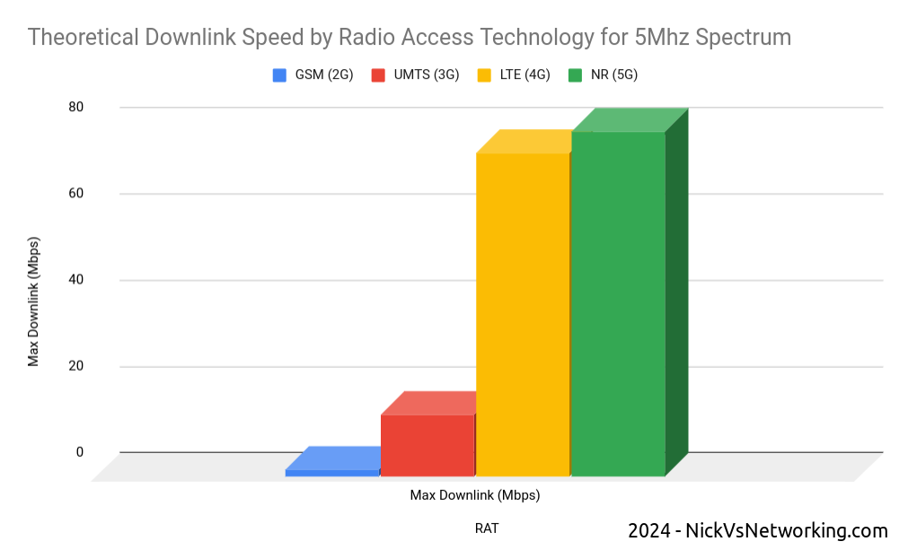
Spectrum is both finite and expensive, so MNOs must find the most efficient way to use that spectrum, to squeeze the most possible value out of it.
In rough numbers, we can say we get 5x the spectral efficiency by moving from 3G to 4G. This means we can carry 5.2x more with the same spectrum on 4G than we can on 3G – A very compelling reason to upgrade.
The like-for-like spectral efficiency of 5G is not significantly greater than that of LTE.
In numbers the same 5Mhz of spectrum we refarmed from UMTS (3G) to 4G (LTE) provided a 5x gain in efficiency to deliver 75Mbps on LTE. The same configuration refarmed to 5G-NR would provide 80Mbps.
Refarming spectrum from 4G (LTE) to 5G (NR) only provides a 6% increase in spectral efficiency.
While 6% is not nothing, if refarmed to a 5G standalone network, the spectrum can no longer be used by LTE only devices (Unless Dynamic Spectrum Sharing is used which in itself leads to efficiency losses), which in itself reduces the efficiency and would add additional load to other layers.
The crazy speeds demonstrated by 5G are not due to meaningful increases in efficiency, but rather the ability to use more spectrum, spectrum that operators need to purchase at auction, purchase equipment to utilize and pay to run.
Claim: 5G Standalone Core is Cheaper to operate as it is “Cloud Native”
It has been widely claimed that the shift for the 5G Core Architecture to being “Cloud Native” can provide cost savings.
Operators should regard this in a skeptical manner; after all, we’ve been here before.
Did moving from big-iron to VNFs provide the promised cost savings to operators?
For many operators the shift from hardware to software added additional complexity to the network and increased the headcount to support this.
What were once big-iron appliances dedicated to one job, that sat in the corner and chugged away, are now virtual machines (VNFs). Many operators have naturally found themselves needing a larger team to manage the virtual environment, compared to the size of the team they needed to just to plug power and data into a big box in an exchange before everything was virtualized.
Introducing a “Cloud Native” Kubernetes layer on top of the VNF / virtualization layer, on top of the compute layer, leaves us with a whole lot of layers. All of which require resources to be maintain, troubleshoot and kept running; each layer having associated costs for staffing, licensing and support.
Many mid size enterprises rushed into “the cloud” for the promised cost savings only to sheepishly admit it cost more than the expected.
Almost none of the operators are talking about running these workloads in the public cloud, but rather “Private Clouds” built on-premises, using “Cloud Native” best practices.
One of the central arguments about cloud revolves around “elastic scaling” where the network can automatically scale to match demand; think extra instances spun up a times of peak demand and shut down when the demand drops.
I explain elastic scaling to clients as having to move people from one place to another. Most of the time, I’m just moving myself, a push bike is fine, or I’ve got a 4 seater car, but occasionally I’ll need to move 25 people and for that I’d need a bus.
If I provide the transportation myself, I need to own a bike, a car and a bus.
But if use the cloud I can start with the push bike, and as I need to move more people, the “cloud” will provide me the vehicle I need to move the people I need to move at that moment, and I’ll just pay for the time I need the bus, and when I’m done needing the bus, I drop back to the (cheaper) push bike when I’m not moving lots of people.
While telecom operators are going to provide the servers to run this in “On-prem-cloud”, they need to dimension for the maximum possible load. This means they need to own a bike/car/bus, even if they’re not using it most of the time, and there’s really no cost savings to having a bus but not using it when you’re not paying by the hour to hire it.
Infrastructure aside, introducing a Standalone 5G Core adds another core network to maintain. Alongside the Circuit Switched Core (MSC/GGSN/SGSN) serving 2G/3G subscribers, Evolved Packet Core serving 4G (LTE) and 5G-NSA subscribers, adding a 5G Standalone Core to for the 5G-SA subscribers served by the 5G SA cells, is going to be more work (and therefore cost).
While the majority of operators have yet to turn off their 2G/3G core networks, introducing another core network to run in parallel is unlikely to lead to any cost savings.
Claim: Upgrading now can save money in the Future / Future Proofing
Life cycles of telecommunications are two fold, one is the equipment/platform life cycle (like the RAN components or Core network software being used to deliver the service) the other is the technology life cycle (the generation of technology being used).
The technology lifecycles in telecommunications are vastly longer than that for regular tech.
GSM (2G) was introduced into the UK in 1991, and will be phased out starting in 2033, a 42 year long technology life cycle.
No vendor today could reasonably expect the 5G hardware you deploy in 2024 to still be in production in 2066 – The platform/equipment life cycle is a lot shorter than the technology life cycle.
Operators will to continue relying on LTE (4G) well into the late 2030s.
I’d wager that there is not a single piece of equipment in the Vodafone UK GSM network today, that was there in 1991. I’d go even further to say that any piece of equipment in the network today, didn’t even replace the 1991 equipment, but was probably 3 or 4 generations removed from the network built in 1991.
For most operators, RAN replacements happen between 4 to 7 years, often with targeted augmentation / expansion as needed in the form of adding extra layers / sectors between these times.
The question operators should be asking is therefore not what will I need to get me through to 2066, but rather what will I need to get to 2030?
The majority of operators outside the US today still operate a 2G or 3G network, generally with minimal bandwidth to support legacy handsets and devices, while the 4G (LTE) network does most of the heavy lifting for carrying user traffic. This is often with the aid of an additional 5G-NSA (Non-Standalone) layer to provide additional capacity.
Is there a cost saving angle to adding support for 5G-Standalone in addition to 2G/3G/4G (LTE) and 5G (Non-Standalone) into your RAN?
A logical stance would be that removing layers / technologies (such as 2G/3G sunsetting) would lead to cost savings, and adding a 5G Standalone layer would increase cost.
All of the RAN solutions on the market today from the major vendors include support for both Standalone 5G and Non Standalone, but the feature licensing for a non-standalone 5G is generally cheaper than that for Standalone 5G.
The question operators should be asking is on what timescale do I need Standalone 5G?
If you’ve rolled out 5G-NSA today, then when are you looking to sunset your LTE network? If the answer is “I hope to have long since retired by that time”, then you’ve just answered that question and you don’t need to licence / deploy 5G-SA in this hardware refresh cycle.
Other Cost Factors
Roaming: The majority of roaming traffic today relies on 2G/3G for voice. VoLTE roaming is (finally) starting to establish a foothold, but we are a long way from ubiquitous global roaming for LTE and VoLTE, and even further away for 5G-SA roaming. Focusing on 5G roaming will enable your network for roaming use by a miniscule number of operators, compared to LTE/VoLTE roaming which covers the majority of the operators in the developed world who can utilize your service.
I decided to split this into 3 posts, next I’ll post the “5G can make us more money” post and finally a “5G because we have to” post. I’ll post that on LinkedIn / Twitter / Mailing list, so stick around, and feel free to trash me in the comments.
Android, being open source, allows us to see how this logic works, and it’s important for operators to understand this logic, as it’s what dictates the behavior in many scenarios.
It’s important to note that I’m not covering Apple here, this information is not publicly available to share for iOS devices, so I won’t be sharing anything on this – Apple has their own ecosystem to handle emergency calling, if you’re from an operator and reading this, I’d suggest getting in touch with your Apple account manager to discuss it, they’re always great to work with.
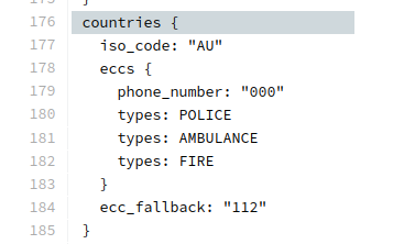
The Android Open Source Project has an “emergency number database”. This database has each of the emergency phone numbers and the corresponding service, for each country.
This file can be read at packages/services/Telephony/ecc/input/eccdata.txt on a phone with engineering mode.
Let’s take a look what’s in mainline Android for Australia:
For example, an American visiting the UK, would have 911 on the Emergency Calling Codes list on their SIM card, but in the UK they dial 999 to reach emergency services.
There’s two angles to this, the first is if a roamer dials the emergency calling code of their home country, the other is if they dial the emergency calling code of the country they are in.
Let’s look at the first scenario, where the roamer dials the emergency calling code of their home country.
If our American in the UK abroad dials 911, that number is on the ECC list on the SIM, it’s still flagged as an emergency call, and just goes out with the standard urn:service:sos URN – The network never sees 911 or 999, just that it’s an SOS call that goes to the PSAP.
In this scenario, the fact the dialled number is not passed to the network is actually a positive, we get the intent that the user wants to reach emergency services, and route based on this.
But what if our American friend in need dials 999? That’s the correct number for the end user to dial in the UK after all, but if that’s not in their ECC list on the SIM / device, it’d go through as a regular call right?
If the call does not get flagged as an emergency call on the UE this has its own set of complications and considerations:
S8-Home Routing for VoLTE means that as the UE doesn’t know this is an emergency call, the call will get routed back to the home network. This means the call doesn’t go to the E-CSCF in the visited network, and would probably just get a message saying the number they’ve dialed is unavailable, this would be exactly as if they dialed 999 at home in the US.
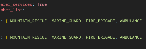
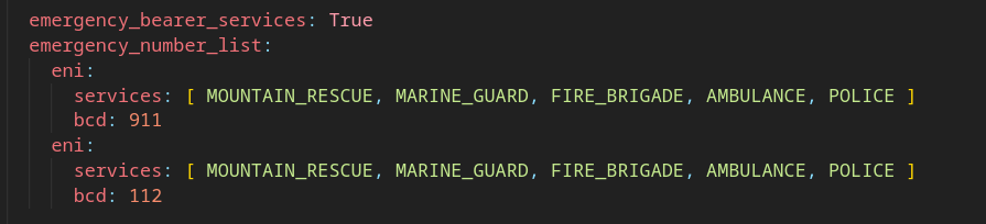
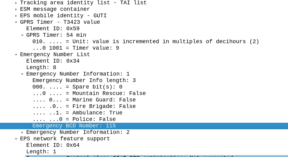
But we have a fix for this! On each MME we can set a list of emergency numbers, which would allow our Britt’s phone to know on this network, what the emergency calling codes are, and route the 999 call to the local PSAP, rather than home routing it.
This information is jammed into the Emergency Number List IE in the NAS Attach Accept body.
This means our American visitor in the UK, would know about 999 from the ECC list configured in the roaming operator’s MME.
The purpose of this information element is to encode emergency number(s) for use within the country where the IE is received.
3GPP TS 24.008: 10.5.3.13 – Emergency Number List
Where this becomes more problematic is unauthenticated emergency calling.
For example, a our American visiting the UK, that is not roaming dials 999.
We’ll assume the UK and US operator don’t have a VoLTE roaming agreement because they’ve been kicking the can down the road when it comes to VoLTE roaming… This is super common scenario – last numbers I saw on this were last year with ~50 bilateral VoLTE agreements in place worldwide.
Because the phone is not attached to a local MME, the handset does not know that 999 is an emergency calling code (because it’s not on the SIM), after all, the only way it can get the Emergency Number List is from an MME, and not having been attached to an MME, means the phone does not have the ECC list for the country, so the the handset does not begin the emergency attach procedure to make the call.
Common sense prevails here, on the majority of phones and the majority of SIM profiles, codes like 112 or 911 are treated as emergency calls, but more obscure numbers, such as dialing 999 in the UK or 10111 for South African Police on a handset with US firmware, are not guaranteed to work. Generally dialing the Emergency Calling code in the home network would get you through to some emergency services (although as we talked about in the last post, this might get you routed to the wrong agency in countries where each agency has their own number).
A better way forward?
These days I don’t dial much (apart from if I’m making adjustments on the Step-by-Step exchange), when I call people I do it from contacts, hyperlinks, etc.
There is mountains of research to suggest that asking people to remember codes and phone numbers, is a struggle. A tourist who finds themselves in Tunisia in need of assistance, is unlikely to remember that it’s 190 for an Ambulance, and 198 for Fire.
Perhaps the ECC list on a phone should populate a page of icons from the emergency page on the phone, with the universal icon for each agency, that sends to the URN for that service type?
Countries with a single PSAP could have the URNs for each service type routed to the same place, while countries with seperated PSAPs for each service type, can route accordingly.
Likewise if a country does have a centralised PSAP for all call types, knowing the type that is selected would be useful, for example if the user has pressed fire and is not responsive when the call is answered, the best unit to dispatch would probably be a fire engine.
A lot of countries have a single point of contact for emergency services; in Europe you’d call 112 in an emergency, 000 in Australia or 911 in the US. Calling this number in the country will get you the emergency services.
This means a caller can order an ambulance for smoke inhalation, and the fire brigade, in one call.
But that’s not the case in every country; many countries don’t have one number for theemergency services, they’ve got multiple; a phone number for police, a different number for fire brigade and a different number for an ambulance.
For example, in Brazil if you need the police, you call 190, while a for example, uses 193 as the emergency number for the fire department, the police can be reached at 190 or 191 depending on if it’s road policing or general, and medical emergencies are covered by 192. Other countries have similar setups.
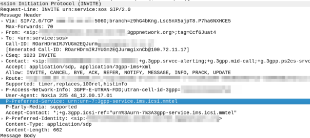
This is all well and good if you’re in Brazil, and you call 192 for an ambulance, the phone sends a SIP INVITE with a Request URI of sip:[email protected], because we can put a rule into our E-CSCF to say if the number is 192 to route it to the answer point for ambulances – But that’s not often the case on emergency calls.
In IMS, handsets generally detect the number dialed is on the Emergency Calling Code (ECC) list from the USIM Card.
The use of the ECC list means the phone knows this is an emergency call, and this is really important. For countries that use AML this can trigger sending of the AML SMS that process, and Emergency Calls should always be allowed to be made, even without credit, a valid SIM card, or even a SIM in the phone at all.
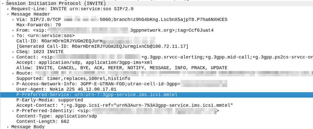
But this comes with a cost; when a user dials 911, the phones doesn’t (generally) send a call to sip:[email protected] like it would with any other dialled number, but rather the SIP INVITE is sent to urn:service:sos which will be routed to the PSAP by the E-CSCF. When a call comes through to these URNs they’re given top priority in the network
This is all well and good in a country where it doesn’t matter which emergency service you called, because all emergency calls route to a single PSAP, but in a country with multiple numbers, it’s really important when you call and ambulance, your call doesn’t get routed to animal control.
That means the phone has to look at what emergency number you’ve dialed, and map the URN it sends the call to to match what you’ve actually requested.
Recently we’ve been helping an operator in a country with a numbering plan like this, and we’ve been finding the limits of the standards here. So let’s start by looking at what the standards state:
IMS Emergency Calling is governed by TS 103.479 which in turn delegates to IETF RFC 5031, but for the calling number to URN translation, it’s pretty quiet.
Let’s look at what RFC 5031 allows for URNs:
urn:service:sos.ambulance
urn:service:sos.animal-control
urn:service:sos.fire
urn:service:sos.gas
urn:service:sos.marine
urn:service:sos.mountain
urn:service:sos.physician
urn:service:sos.poison
urn:service:sos.police
The USIM’s Emergency Calling Codes EF would be the perfect source of this data; for each emergency calling code defined, you’ve got a flag to indicate what it’s for, here’s what we’ve got available on the SIM Card:
Bit 1 Police
Bit 2 Ambulance
Bit 3 Fire Brigade
Bit 4 Marine Guard
Bit 5 Mountain Rescue
Bit 6 manually initiated eCall
Bit 7 automatically initiated eCall
Bit 8 is spare and set to “0”
So these could be mapped pretty easily you’d think, so if the call is made to an Emergency Calling Code flagged with Bit 4, the URN would go to urn:service:sos.mountain.
Alas from our research, we’ve found most OEMs send calls to the generic urn:service:sos, regardless of the dialled number and the ECC flags that are set on the SIM for that number.
One of the big chip vendors sends calls to an ECC flagged as Ambulance to urn:service:sos.fire, which is totally infuriating, and we’ve had to put a rule in our E-CSCF to handle this if the User Agent is set to one of their phones.
Is there room for improvement here? For sure! Emergency calling is super important, and time is of the essence, while animal control can probably transfer you to an ambulance, an emergency is by very nature time sensitive, and any time wasted can lead to worse outcomes.
While carrier bundles from the OEMs can handle this, the global ability to take any phone, from any country and call an emergency number is so important, that relying on a country-by-country approach here won’t suffice.
What could we do as an industry to address this?
Acknowledging that not all countries have a single point of contact for emergency service, introducing a simple mechanism in the UE SIP message to indicate what number (Emergency Calling Code) the user actually dialled would be invaluable here.
URNs are important, but knowing the dialed number when it comes to PSAP routing, is so important – This wouldn’t even need to be its own SIP header, it could just be thrown into the Contact header as another parameter.
Highly developed markets are often the first to embrace new tech (for us this means VoLTE and VoNR), but this means that these issues seen by less developed markets won’t appear until long after the standard has been set in stone, and often countries like this aren’t at the table of the standards bodies to discuss such requirements.
This easy, reasonable update to the standard, has the potential to save lives, and next time this comes up in a working group I’ll be advocating for a change.
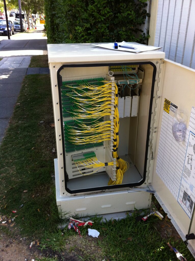
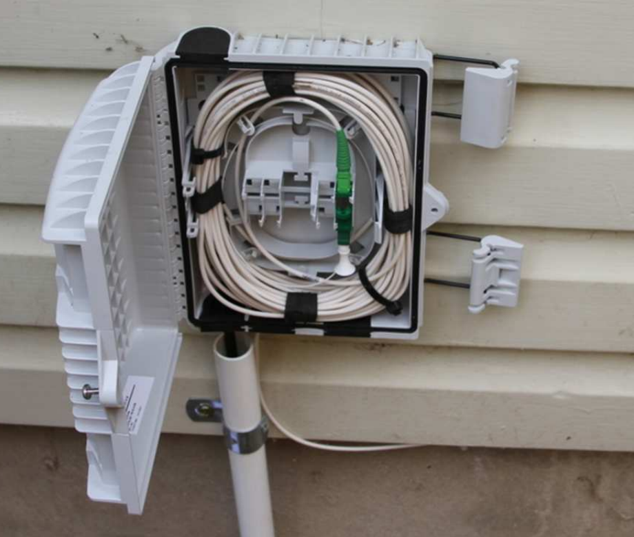
At long last, more and more Australians are going to have access to fibre based access to the NBN, and this seemed like as good an excuse than any to take a deep dive into how NBN’s GPON based fibre services are delivered to homes.
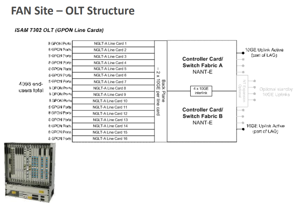
Let’s start in your local exchange where you’ll likely find a Nokia (Well, probably Alcatel-Lucent branded) 7210 SAS-R access aggregation switch, which is where NBN’s transmission network ends, and the access network begins.
It in turn spits out a 10 gig interface to feed the Optical Line Terminal (OLT), which provides the GPON services, each port on the OLT is split out and can feed 32 subscribers.
In NBN’s case, Nokia (Alcatel-Lucent) 7302, and rather than calling it an OLT, they call it a “FAN” or “Fibre Access Node” – Seemingly because they like the word node.
Each of the Nokia 7302s has at least one NGLT-A line card, which has 8 GPON ports. Each of the 8 ports on these cards can service 32 customers, and is fed by 2x 10Gbps uplinks to two 7210 SAS-R aggregation switches.
The chassis supports up to 16 cards, 8 ports each, 32 subs per port, giving us 4096 subscribers per FAN.
In some areas, FANs/OLTs aren’t located in an exchange but rather in a street cabinet, called a Temporary Fibre Access Node – Although it seems they’re very permanent.
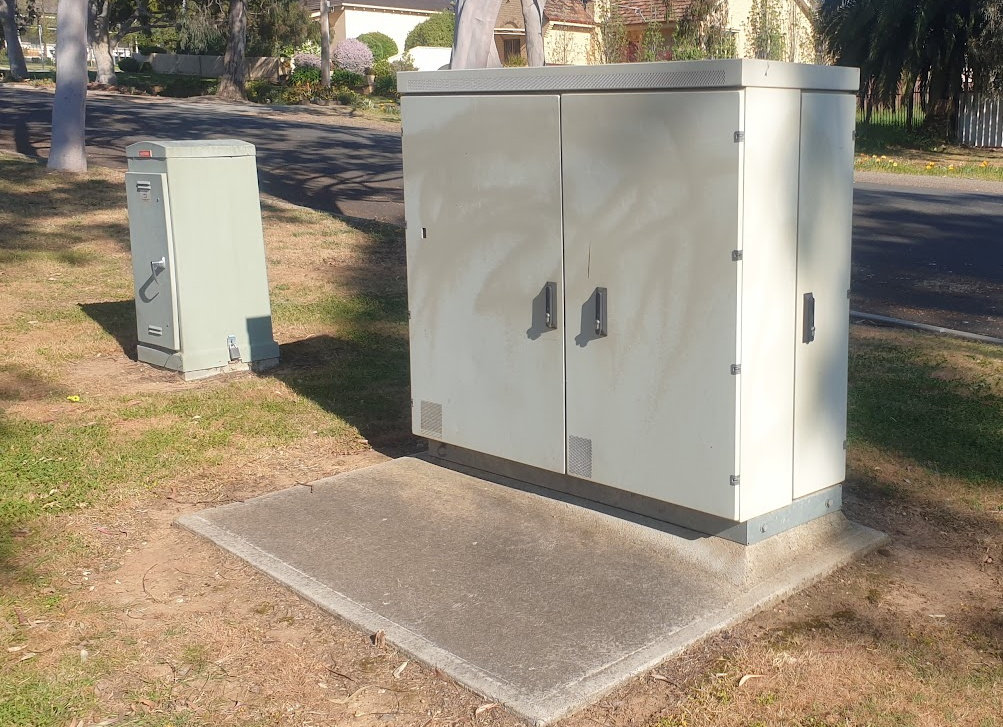
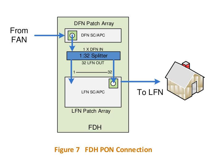
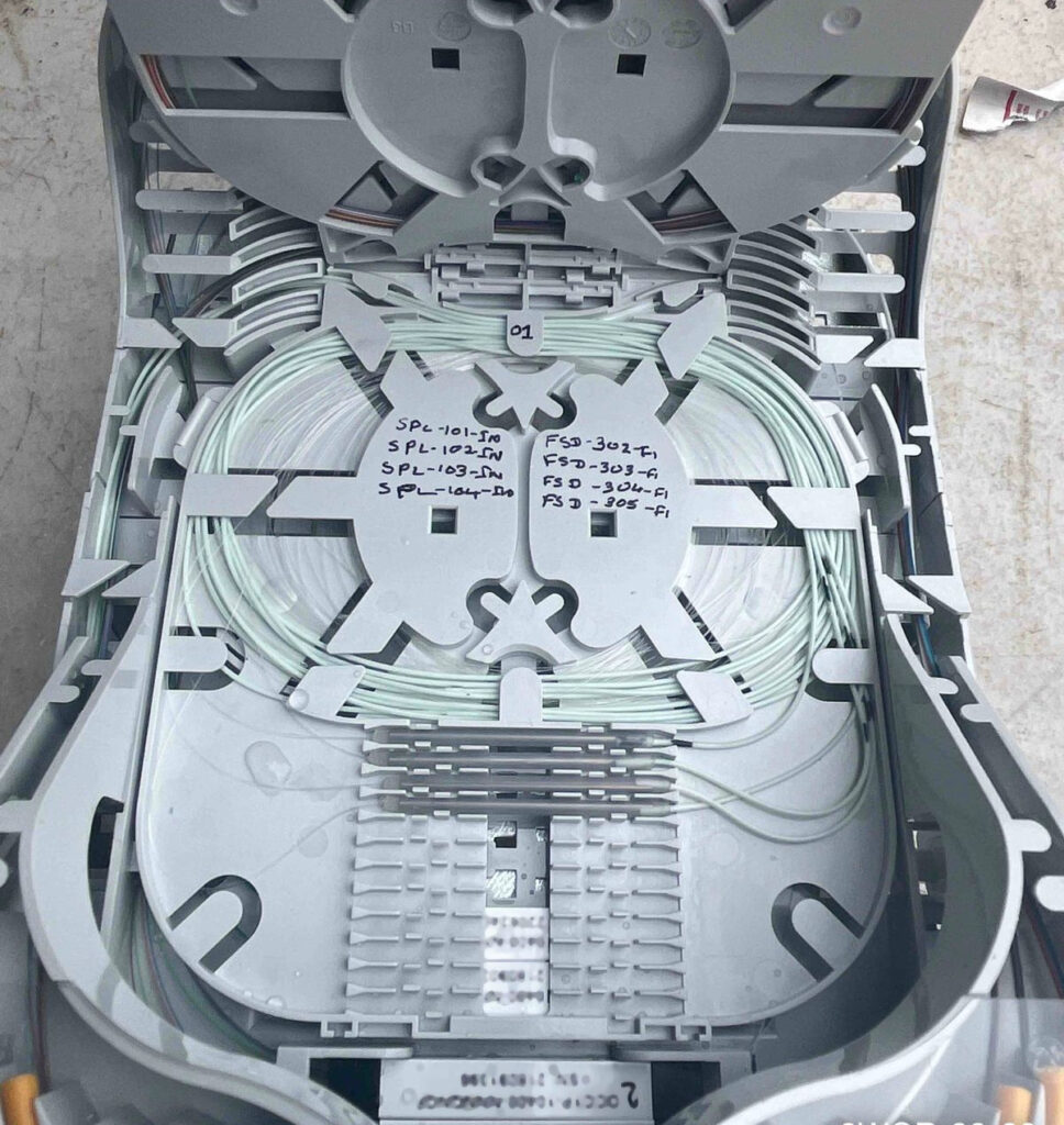
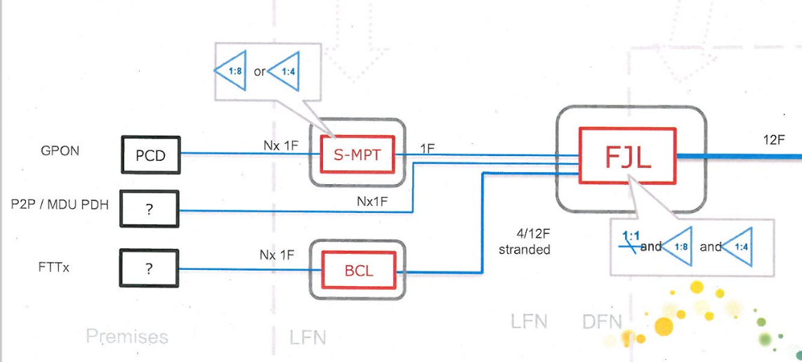
In reality, each port on the OLT/FAN goes out Distribution Fibre Network or DFN which links the ports on the OLTs to a distribution cabinet in the street, known as as a Fibre Distribution Hub, or FDH.
If you look in FTTH areas, you’ll see the FDH cabinets. The FDH is essentially a roadside optical distribution frame, used to cross connect cables from the Distribution Fibre Network (DFN) to the Local Fibre Network (LFN), and in a way, you can think of it as the GPON equivalent of a pillar, except this is where we have our optical splitters.
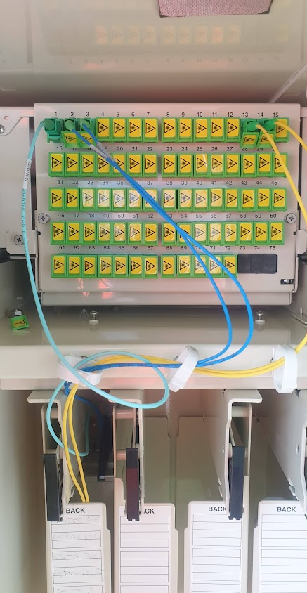
Remember when we were talking about the FAN/OLT how one port could serve 32 subscribers? We do that with a splitter, that takes one fibre from the DFN that runs to the FAN, and gives us 32 fibres we can could connect to an ONT onto to get service.
Inside the FDH showing the Distribution Fibre Network (DFN) connecting to the optical splitters belowDistribution Fibre Network with up to 576 fibres running out and down streets, with parking below
The FDH cabinets are made by Corning (OptiTect 576 fibre pad mounted cabinets) and you can see in the top right the Aqua cables go to the Distribution Fibre Network, and hanging below it on the right are the optical splitters themselves, which split the one fibre to the FAN into 32 fibres each on SC connectors.
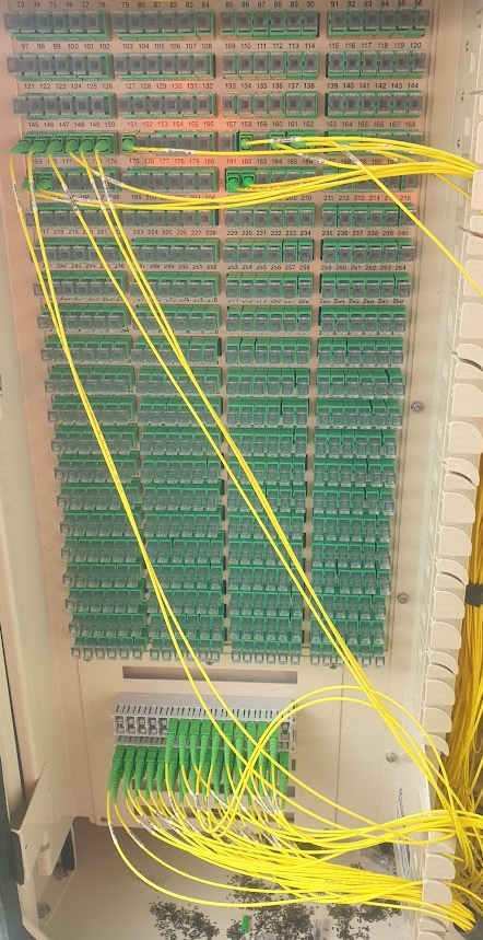
These are then patched to the Local Fibre Network on the left hand side of the cabinet, where there’s up to 576 ports running across the suburb, and a “Parking” panel at the bottom where the unused ports from the splitter can be left until you patch the to the DFN ports above.
The FDH cabinets also offer “passthrough” allowing a fibre to from the FAN to be patched through to the DFN without passing through the GPON splitter, although I’m not clear if NBN uses this capability to deliver the NBN Business services.
But having each port in the FDH going to one home would be too simple; you’d have to bring 576 individually sheathed cables to the FDH and you’d lose too much flexibility in how the cable plant can be structured, so instead we’ve got a few more joints to go before we make it to your house.
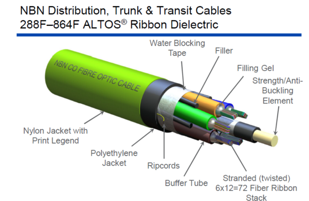
From the FDH cabinet we go out into the Local Fibre Network, but NBN has two variants of LFN – LFN and Skinny LFN. The traditional LFN uses high-density ribbon fibres, which offer a higher fibre count but is a bit tricker to splice/work with. The Skinny LFN uses lower fibre count cables with stranded fibres, and is the current preferred option.
The original LFN cables are ribbon fibres and range from 72 to 288 fibre counts, but I believe 144 is the most common.
These LFN cables run down streets and close to homes, but not directly to lead in cables and customer houses.
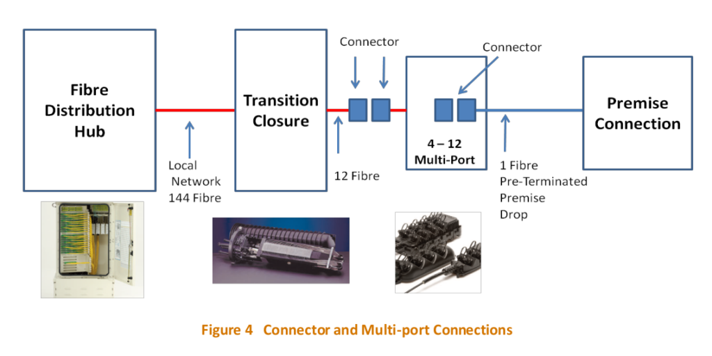
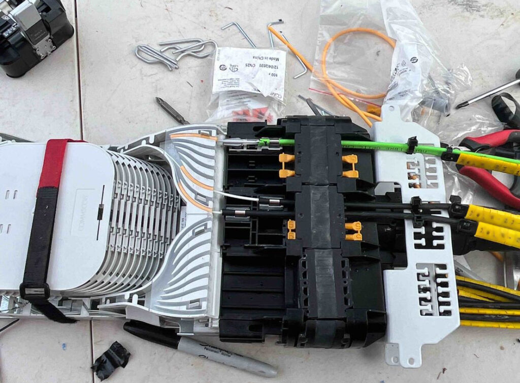
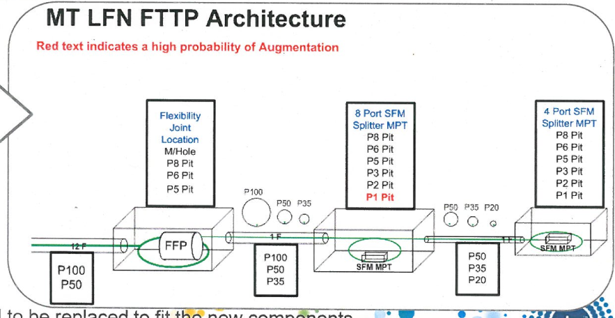
These run to “Transition Closures” (Older NBN) or “Flexibility Joint Locations” (FJLs – Newer NBN)
While researching this I saw references to “Breakout Joint Locations” (BJLs) which are used in FTTC deployments, and are a Tenio B6 enclosure for 2x 12 Fibers and 4x 1 Fibers with a 1×4 splitter.
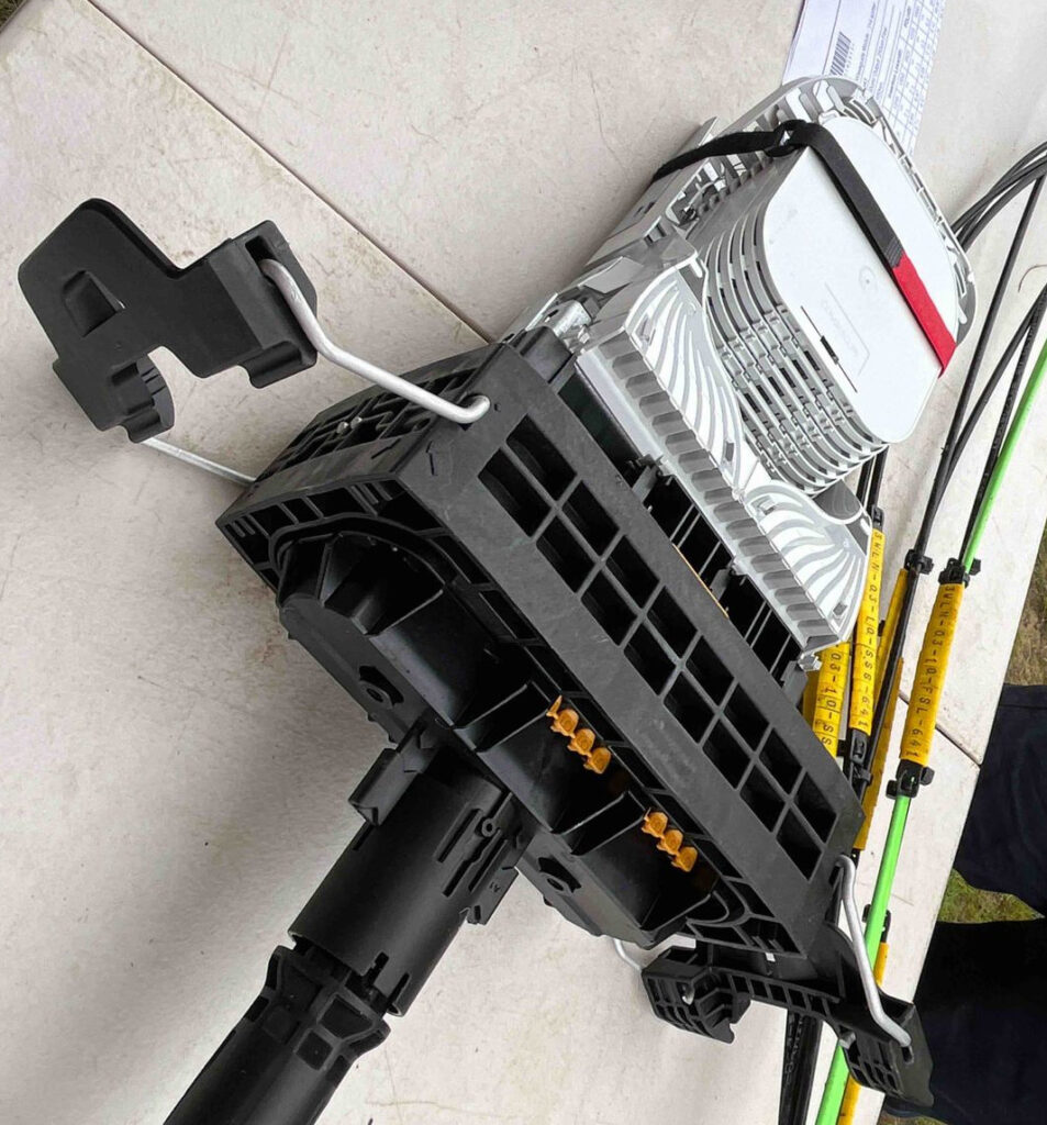
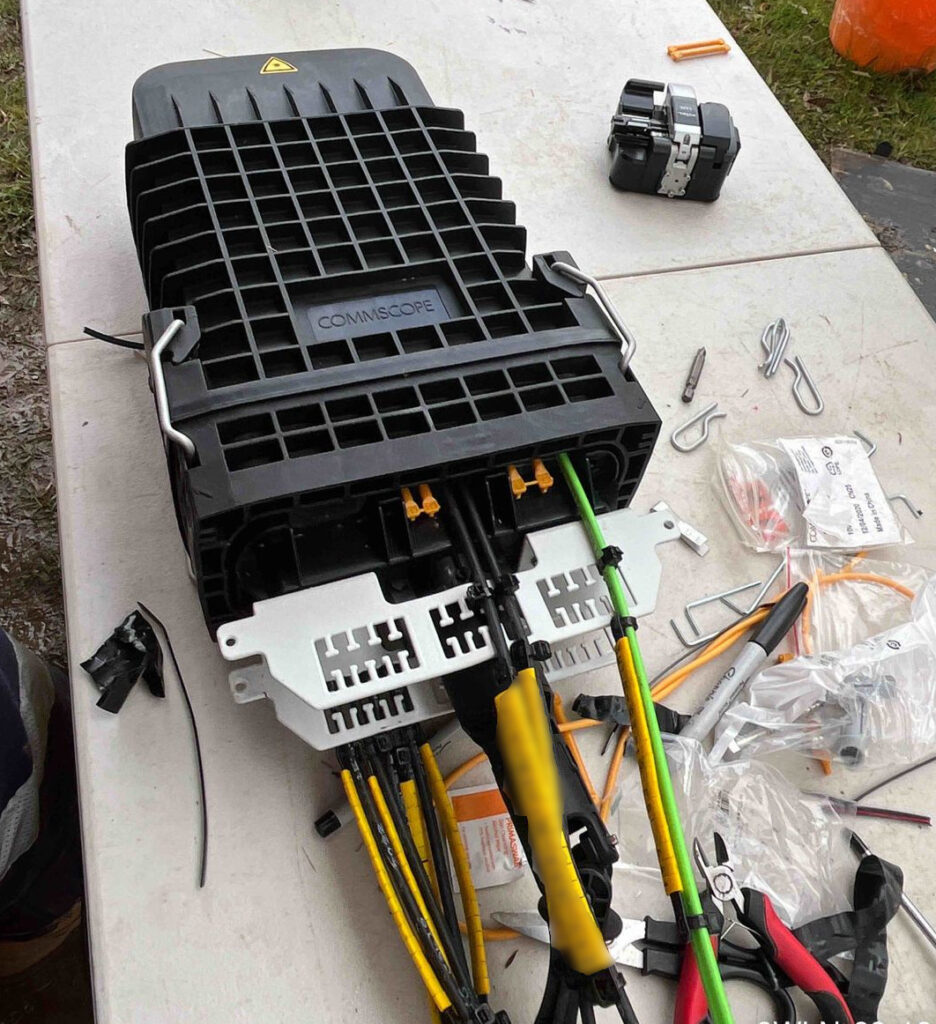
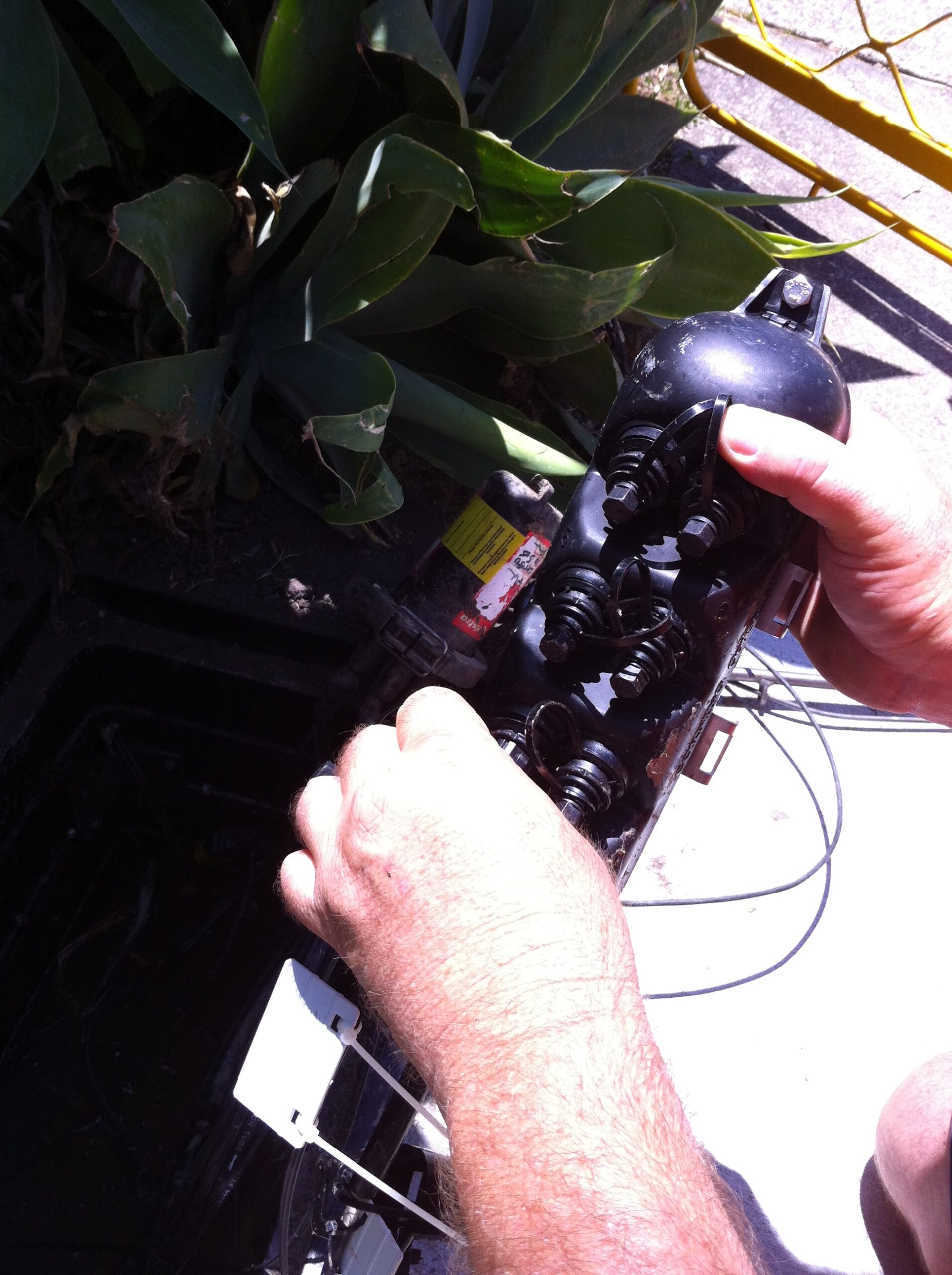
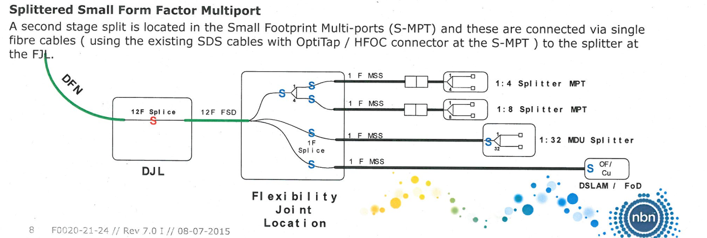
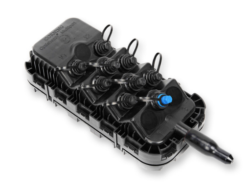
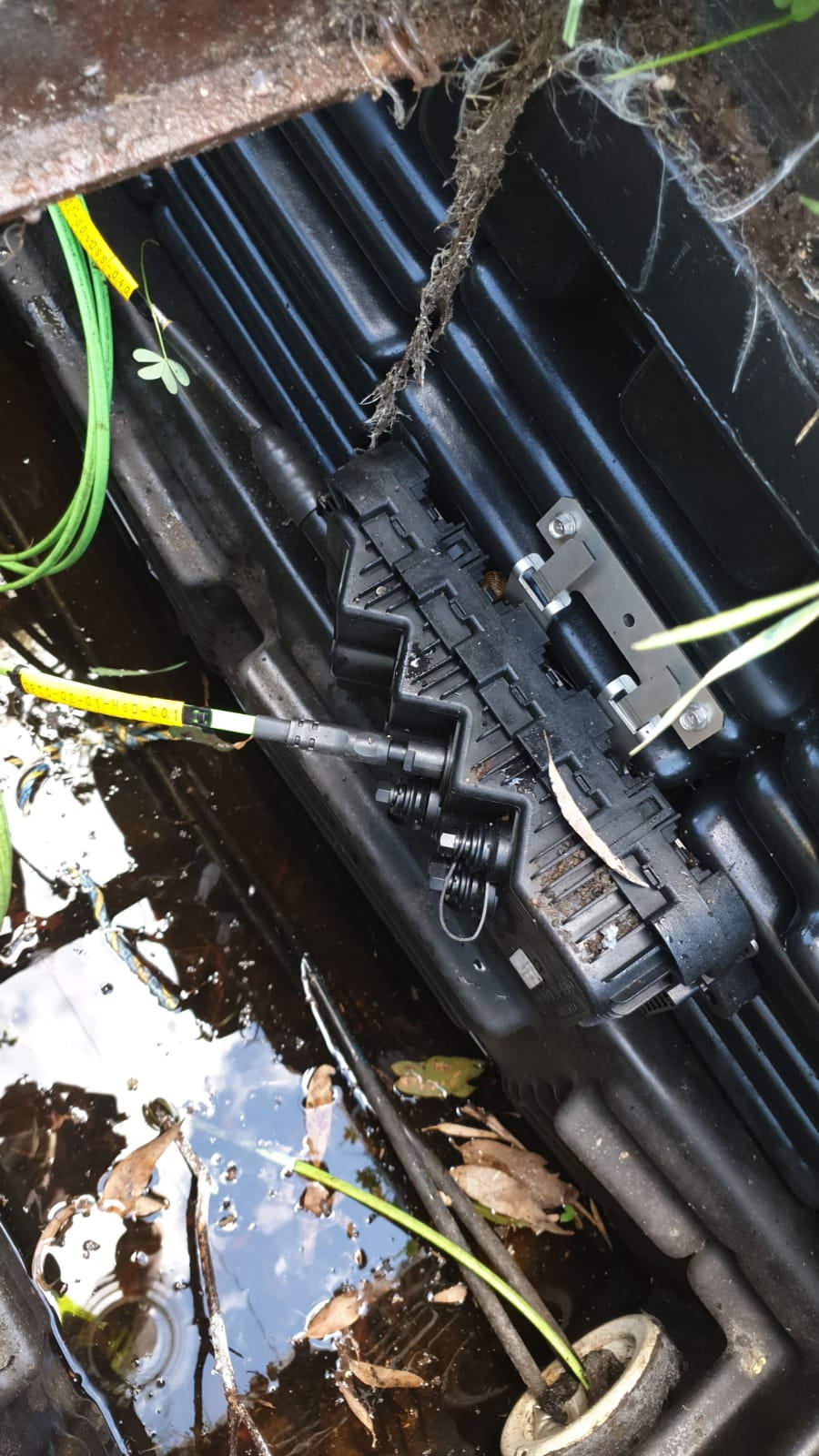
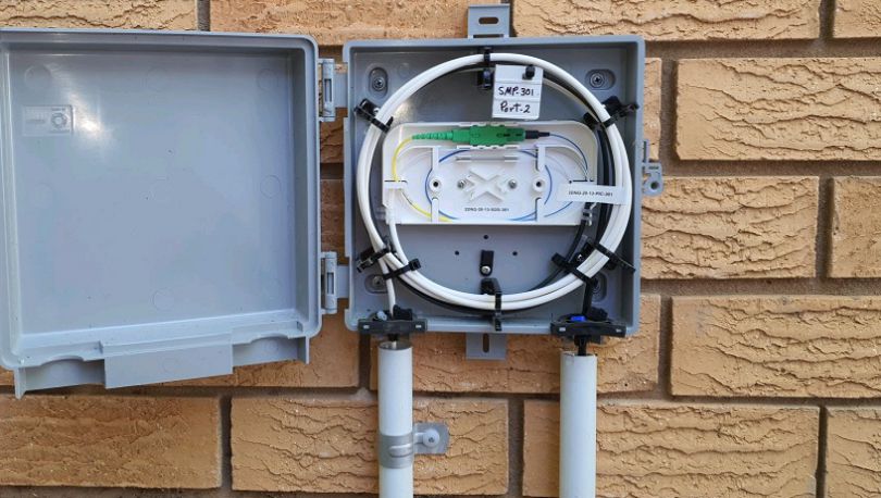
The FJLs are TE Systems’ (Now Commscope) Tenio range of fibre splice closures, and they’re use to splice the high fibre count cable from from the FDH cabinets into smaller 12 fibre count cables that run to multiple “Splitter Multi Ports” or “SMPs” in pits outside houses, and can contain splitters factory installed.
Sealed NBN FJLOpen NBN FJLReassembled NBN FJLFJL in situ in pitNeat open FJL
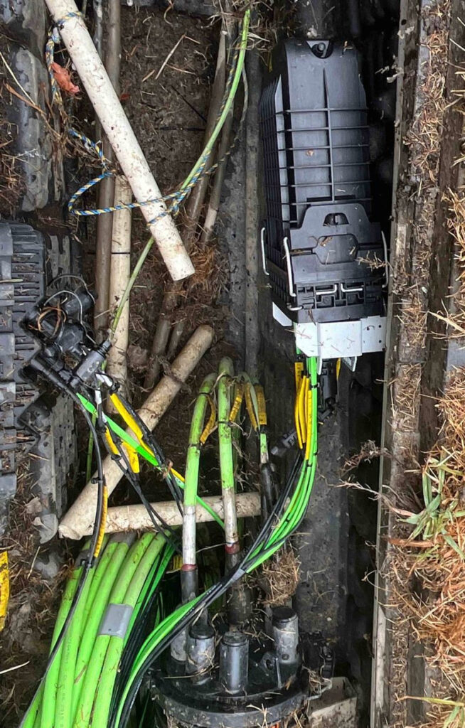
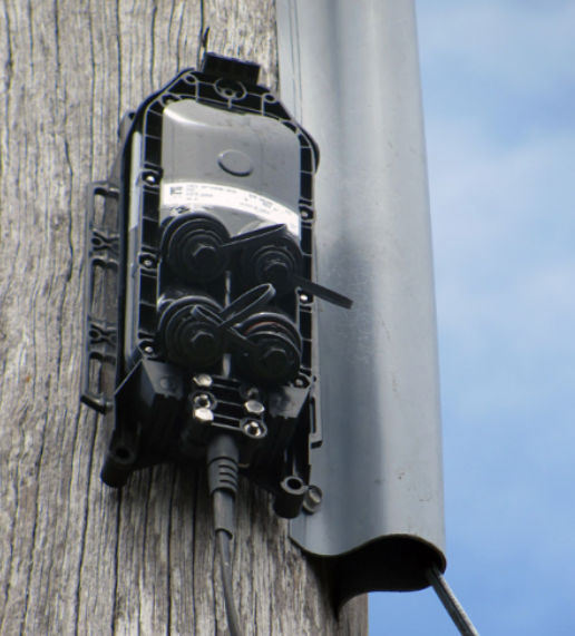
The splitters, referred to as “Multiports” or “SMPs” are Corning’s OptiSheath MultiPort Terminals, and they’re designed and laid out in such a way that the tech can activate a service, without needing to use a fusion splicer.
Due to the difficulty/cost in splicing fibre in pits for a service activation, NBNco opted to go from the FJL to the SMPs, where a field tech can just screw in a weatherproof fibre connector lead in to the customer’s premises.
During installation / activation callouts, the tech is assigned an SMP in the pit near the customer’s house, and a port on it. This in turn goes to the FJL and onto FDH cabinet as we just covered, but that patching/splicing for that is already done, so the tech doesn’t need to worry about that.
SMP in pitCorning OptiSheath Multiport SplitterSMP in a pit
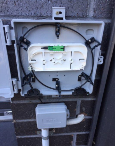
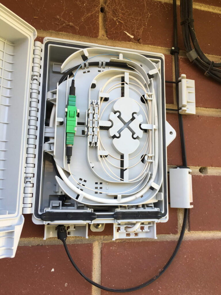
The tech just plugs in a pre-terminated lead in cable with a weatherproof fibre end, and screws it into the allocated port on the SMP, then hauls the other end of the lead in cable to the Premises Connection Device (Made by Madison or Tyco), located on the wall of the customer’s house.
TC000006252
The customer end of the lead in cable may be a pre terminated SC connector, or may get mechanically spliced onto a premade SC pigtail. In either case, they both terminate onto an SC male connector, which goes into an SC-SC female coupler inside the PCD.
Next is the customer’s internal wiring, again, preterm cable is used, to run between the PCD and the First Fibre Wall Outlet inside the house. This preterm cable join the lead in cable inside the PCD on the SC-SC female coupler, to join to the lead in.
Inside the house we have the “Network Termination Device” (NTD), which is a GPON ONT, is where the fibre from the street terminates and is turned into an Ethernet handoff to the customer. NBN has been through a few models of NTD, but the majority support 2x ATA ports for analog phones, and the option for an external battery backup unit to keep the device powered if mains power is lost.
Phew! That’s what I’ve been able to piece together from publicly available documentation, some of this may be out of date, and I can see there’s been several revisions to the LFN / DFN architectures over the years, if there’s anything I have incorrect here, please let me know!
In the cellular world, subscribers are charged for data from the IP, transport and applications layers; this means you pay for the IP header, you pay for the TCP/UDP header, and you pay for the contents (the cat videos it contains).
This also means if an operator moves mobile subscribers from IPv4 to IPv6, there’s an extra 20 bytes the customer is charged for for every packet sent / received, which the customer is charged for – This is because the IPv6 header is longer than the IPv4 header.
In most cases, mobile subs don’t get a choice as to if their connection is IPv4 or IPv6, but on a like for like basis, we can say that if a customer moves is on IPv6 every packet sent/received will have an extra 20 bytes of data consumed compared to IPv4.
This means subscribers use more data on IPv6, and this means they get charged for more data on IPv6.
For IoT applications, light users and PAYG users, this extra 20 bytes per packet could add up to something significant – But how much?
We can quantify this, but we’d need to know the number of packets sent on average, and the quantity of the data transferred, because the number of packets is the multiplier here.
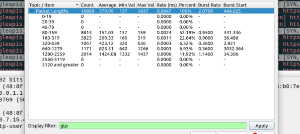
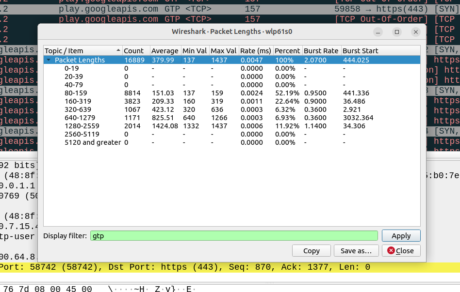
So for starters I’ve left a phone on the desk, it’s registered to the network but just sitting in Idle mode – This is an engineering phone from an OEM, it’s just used for testing so doesn’t have anything loaded onto it in terms of apps, it’s not signed into any applications, or checking in the background, so I thought I’d try something more realistic.
So to get a clearer picture, I chucked a SIM in my regular everyday phone I use personally, registered it to the cellular lab I have here. For the next hour I sniffed the GTP traffic for the phone while it was sitting on my desk, not touching the phone, and here’s what I’ve got:
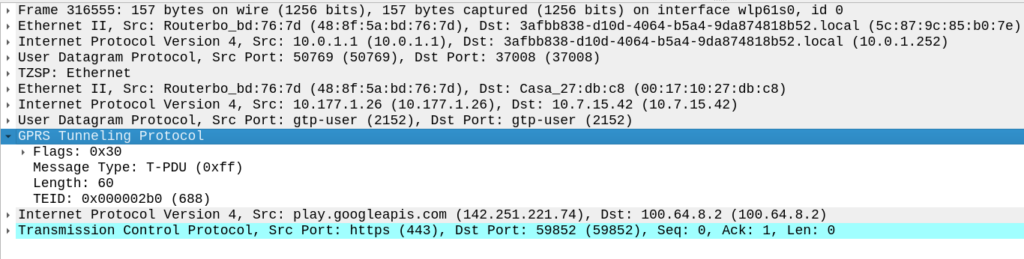
Overall the PCAP includes 6,417,732 bytes of data, but this includes the transport and GTP headers, meaning we can drop everything above it in our traffic calculations.
For this I’ve got 14 bytes of ethernet, 20 bytes IP, 8 bytes UDP and 5 bytes for TZSP (this is to copy the traffic from the eNB to my local machine), then we’ve got the transport from the eNB to the SGW, 14 bytes of ethernet again, 20 bytes of IP , 8 bytes of UDP and 8 bytes of GTP then the payload itself. Phew. All this means we can drop 97 bytes off every packet.
We have 16,889 packets, 6,417,732 bytes in total, minus 97 bytes from each gives us 1,638,233 of headers to drop (~1.6MB) giving us a total of 4.556 MB traffic to/from the phone itself.
This means my Android phone consumes 4.5 MB of cellular data in an hour while sitting on the desk, with 16,889 packets in/out.
Okay, now we’re getting somewhere!
So now we can answer the question, if each of these 16k packets was IPv6, rather than IPv4, we’d be adding another 20 bytes to each of them, 20 bytes x 16,889 packets gives 337,780 bytes (~0.3MB) to add to the total.
If this traffic was transferred via IPv6, rather than IPv4, we’d be looking at adding 20 bytes to each of the 16,889 packets, which would equate to 0.3MB extra, or about 7% overhead compared to IPv4.
But before you go on about what an outrage this IPv6 transport is, being charged for those extra bytes, that’s only one part of the picture.
There’s a reason operators are finally embracing IPv6, and it’s not to put an extra 7% of traffic on the network (I think if you asked most capacity planners, they’d say they want data savings, not growth).
IPv6 is, for lack of a better term, less rubbish than IPv4.
There’s a lot of drivers for IPv6, and some of these will reduce data consumption. IPv6 is actually your stuff talking directly to the remote stuff, this means that we don’t need to rely on NAT, so no need to do NAT keepalives, and opening new sessions, which is going to save you data. If you’re running apps that need to keep a connection to somewhere alive, these data savings could negate your IPv6 overhead costs.
Will these potential data savings when using IPv6 outweigh the costs?
That’s going to depend on your use case.
If you’ve extremely bandwidth / data constrained, for example, you have an IoT device on an NTN / satellite connection, that was having to Push data every X hours via IPv4 because you couldn’t pull data from it as it had no public IP, then moving it to IPv6 so you can pull the data on the public IP, on demand, will save you data. That’s a win with IPv6.
If you’re a mobile user, watching YouTube, getting push notifications and using your phone like a normal human, probably not, but if you’re using data like a normal user, you’ve probably got a sizable data allowance that you don’t end up fully consuming, and the extra 20 bytes per packet will be nothing in comparison to the data used to watch a 2k video on your small phone screen.
Ask someone with headphones and a lanyard in the halls of a datacenter what transport does DNS use, there’s a good chance the answer you’d get back is UDP Port 53.
But not always!
In scenarios where the DNS response is large (beyond 512 bytes) a DNS query will shift over to TCP for delivery.
How does the client know when to shift the request to TCP – After all, the DNS server knows how big the response is, but the client doesn’t.
The answer is the Truncated flag, in the response.
The DNS server sends back a response, but with the Truncated bit set, as per RFC 1035:
TC TrunCation – specifies that this message was truncated due to length greater than that permitted on the transmission channel.
RFC 1035
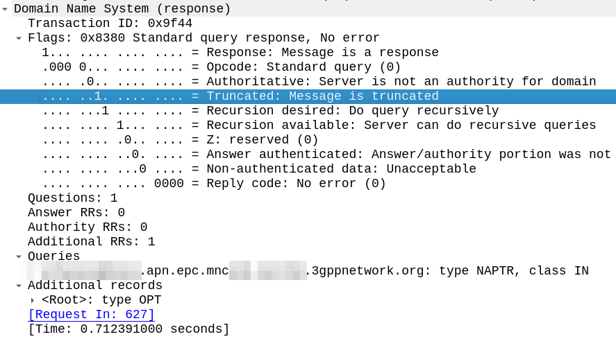
Here’s an example of the truncated bit being set in the DNS response.
The DNS client, upon receiving a response with the truncated bit set, should run the query again, this time using TCP for the transport.
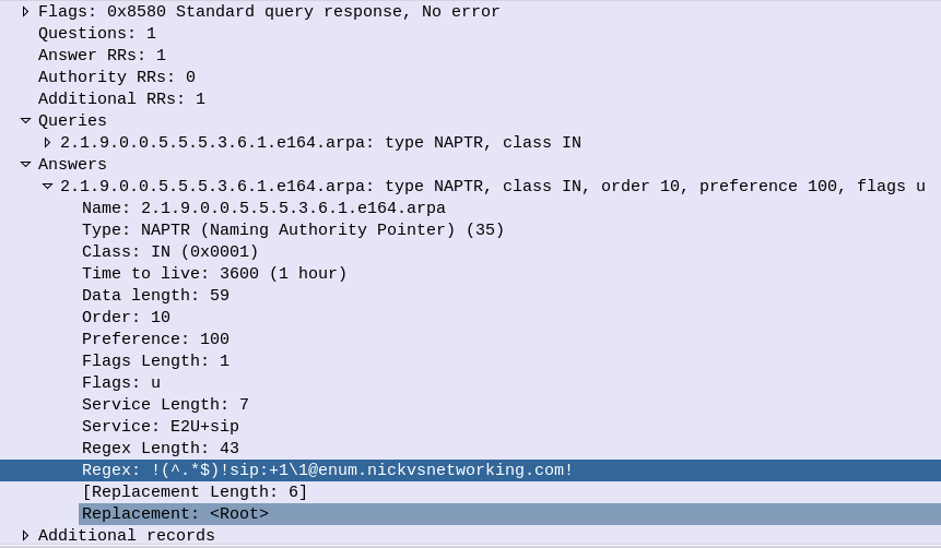
One prime example of this is DNS NAPTR records used for DNS in roaming scenarios, where the response can quite often be quite large.
If it didn’t move these responses to TCP, you’d run the risk of MTU mismatches dropping DNS. In that half of my life has been spent debugging DNS issues, and the other half of my life debugging MTU issues, if I had MTU and DNS issues together, I’d be looking for a career change…
There’s old joke about standards that the great thing about standards there’s so many to choose from.
SMS wasn’t there from the start of GSM, but within a year of the inception of 2G we had SMS, and we’ve had SMS, almost totally unchanged, ever since.
In a recent Twitter exchange, I was asked, what’s the best way to transport SMS? As always the answer is “it depends” so let’s take a look together at where we’ve come from, where we are now, and how we should move forward.
How we got Here
Between 2G and 3G SMS didn’t change at all, but the introduction of 4G (LTE) caused a bit of a rethink regarding SMS transport.
Early builders of LTE (4G) networks launched their 4G offerings without 4G Voice support (VoLTE), with the idea that networks would “fall back” to using 2G/3G for voice calls.
This meant users got fast data, but to make or receive a call they relied on falling back to the circuit switched (2G/3G) network – Hence the name Circuit Switched Fallback.
Falling back to the 2G/3G network for a call was one thing, but some smart minds realised that if a phone had to fall back to a 2G/3G network every time a subscriber sent a text (not just calls) – And keep in mind this was ~2010 when SMS traffic was crazy high; then that would put a huge amount of strain on the 2G/3G layers as subs constantly flip-flopped between them.
The SGs-AP interface has two purposes; One, It can tell a phone on 4G to fallback to 2G/3G when it’s got an incoming call, and two; it can send and receive SMS.
SMS traffic over this interface is sometimes described as SMS-over-NAS, as it’s transported over a signaling channel to the UE.
This also worked when roaming, as the MSC from the 2G/3G network was still used, so SMS delivery worked the same when roaming as if you were in the home 2G/3G network.
Enter VoLTE & IMS
Of course when VoLTE entered the scene, it also came with it’s own option for delivering SMS to users, using IP, rather than the NAS signaling. This removed the reliance on a link to a 2G/3G core (MSC) to make calls and send texts.
This was great because it allowed operators to build networks without any 2G/3G network elements and build a fully standalone LTE only network, like Jio, Rakuten, etc.
In roaming scenarios, S8 Home Routing for VoLTE enabled SMS to be handled when roaming the same way as voice calls, which made SMS roaming a doddle.
4G SMS: SMS over IP vs SMS over NAS
So if you’re operating a 4G network, should you deliver your SMS traffic using SMS-over-IP or SMS-over-NAS?
Generally, if you’ve been evolving your network over the years, you’ve got an MSC and a 2G/3G network, you still may do CSFB so you’ve probably ended up using SMS over NAS using the SGs-AP interface. This method still relies on “the old ways” to work, which is fine until a discussion starts around sunsetting the 2G/3G networks, when you’d need to move calling to VoLTE, and SMS over NAS is a bit of a mess when it comes to roaming.
Greenfield operators generally opt for SMS over IP from the start, but this has its own limitations; SMS over IP is has awful efficiency which makes it unsuitable for use with NB-IoT applications which are bandwidth constrained, support for SMS over IP is generally limited to more expensive chipsets, so the bargain basement chips used for IoT often don’t support SMS over IP either, and integration of VoLTE comes with its own set of challenges regarding VoLTE enablement.
5G enters the scene (Nsmsf_SMService)
5G rolled onto the scene with the opportunity to remove the SMS over NAS option, and rely purely on SMS over IP (IMS); forcing the industry to standardise on an option alas this did not happen.
This added another option for SMS delivery dependent on the access network used, and the Nsmsf_SMService interface does not support roaming.
Of course if you are using Voice over NR (VoNR) then like VoLTE, SMS is carried in a SIP message to the IMS, so this negates the need for the Nsmsf_SMService.
2G/3G Shutdown – Diameter to replace SGs-AP (SGd)
With the 2G/3G shutdown in the US operators who had up until this point been relying on SMS-over-NAS using the SGs-AP interface back to their MSCs were forced to make a decision on how to route SMS traffic, after the MSCs were shut down.
This landed with SMS-over-Diameter, where the 4G core (MME) communicates over Diameter with the SMSc.
This has adoption by all the US operators, but we’re not seeing it so widely deployed in the rest of the world.
State of Play
Option
Conditions
Notes
MAP
2G/3G Only
Relies on SS7 signaling and is very old Supports roaming
SGs-AP (SMS-over-NAS)
4G only relies on 2G/3G
Needs an MSC to be present in the network (generally because you have a 2G/3G network and have not deployed VoLTE) Supports limited roaming
SMS over IP (IMS)
4G / 5G
Not supported on 2G/3G networks Relies on a IMS enabled handset and network Supports roaming in all S8 Home Routed scenarios Device support limited, especially for IoT devices
Diameter SGd
4G only / 5G NSA
Only works on 4G or 5G NSA Better device support than 4G/5G Supports roaming in some scenarios
Nsmsf_SMService
5G standalone only
Only works on 5GC Doesn’t support roaming
The convoluted world of SMS delivery options
A Way Forward:
While the SMS payload hasn’t changed in the past 31 years, how it is transported has opened up a lot of potential options for operators to use, with no clear winner, while SMS revenues and traffic volumes have continued to fall.
For better or worse, the industry needs to accept that SMS over NAS is an option to use when there is no IMS, and that in order to decommission 2G/3G networks, IMS needs to be embraced, and so SMS over IP (IMS) supported in all future networks, seems like the simple logical answer to move forward.
And with that clear path forward, we add in another wildcard…
But, when you’ve only got a finite resource of bandwidth, and massive latencies to contend with, the all-IP architecture of IMS (VoLTE / VoNR) and it’s woeful inefficiency starts to really sting.
Of course there are potential workarounds here, Robust Header Correction (ROHC) can shrink this down, but it’s still going to rely on the 3 way handshake of TCP, TCP keepalive timers and IMS registrations, which in turn can starve the radio resources of the satellite link.
Even with SMS over 30 years old, we can still expect it to be a part of networks for years to come, even as WhatsApp / iMessage, etc, offer enhanced services. As to how it’s transported and the myriad of options here, I’m expecting that we’ll keep seeing a multi-transport mix long into the future.
For simple, cut-and-dried 4G/5G only network, IMS and SMS over IP makes the most sense, but for anything outside of that, you’ve got a toolbox of options for use to make a solution that best meets your needs.
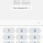
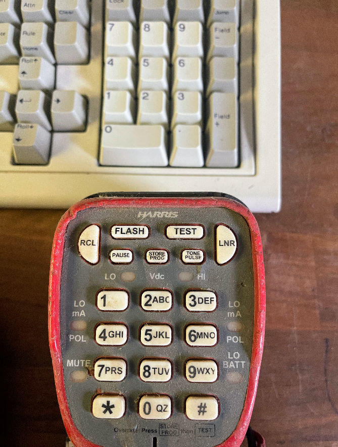
If you’re typing on a full size keyboard there’s a good chance that to your right, there’s a number pad.
The number 5 is in the middle – That’s to be expected, but is 1 in the top left or bottom left?
Being derived from an adding machine keypad, the number pad on a keyboard has a 1 will be in the bottom left, however in the 1950s when telephone keypads were being introduced, only folks who worked in accounting had adding machines.
So when it came time to work out the best layout, the result we have today was a determined through a stack of research and testing by Human Factors Engineering Department of Bell Labs who studied the most efficient layout of keys, and tested focus groups to find the layout that provided the best level of speed and accuracy.
That landed with the 1 in the top left, and that’s what we still have today.
Oddly ATM and Card terminals opted to use the telephone layout, rather than the adding machine layout, while number pads use the adding machine layout.
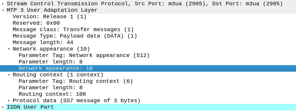
Short one, The other day I needed to add a Network Appearance on an SS7/SS7 M3UA linkset.
Network Appearances on M3UA links are kinda like a port number, in that they allow you to distinguish traffic to the same point code, but handled by different logical entities.
When I added the NA parameter on the Linkset nothing happened.
If you’re facing the same you’ll need to set:
cs7 multi-instance
In the global config (this is the part I missed).
Then select the M3UA linkset you want to change and add the network-appearance parameter:
network-appearance 10
And bingo, you’ll start seeing it in your M3UA traffic:
The Binding Support Function is used in 4G and 5G networks to allow applications to authenticate against the network, it’s what we use to authenticate for XCAP and for an Entitlement Server.
Rather irritatingly, there are two BSF addresses in use:
If the ISIM is used for bootstrapping the FQDN to use is:
bsf.ims.mncXXX.mccYYY.pub.3gppnetwork.org
But if the USIM is used for bootstrapping the FQDN is
bsf.mncXXX.mccYYY.pub.3gppnetwork.org
You can override this by setting the 6FDA EF_GBANL (GBA NAF List) on the USIM or equivalent on the ISIM, however not all devices honour this from my testing.
One of the hyped benefits of a 5G Core Networks is that 5GC can be used for wired networks (think DSL or GPON) – In marketing terms this is called “Wireless Wireline Convergence” (5G WWC) meaning DSL operators, cable operators and fibre network operators can all get in on this sweet 5GC action and use this sexy 5G Core Network tech.
This is something that’s in the standards, and that the big kit vendors are pushing heavily in their marketing materials. But will it take off? And should operators of wireline networks (fixed networks) be looking to embrace 5GC?
Comparing 5GC with current wireline network technologies isn’t comparing apples to apples, it’s apples to oranges, and they’re different fruits.
At its heart, the 3GPP Core Networks (including 5G Core) address one particular use cases of the cellular industry: Subscriber mobility – Allowing a customer to move around the network, being served by different kit (gNodeBs) while keeping the same IP Address.
The most important function of 5GC is subscriber mobility.
This is achieved through the use of encapsulating all the subscriber’s IP data into a GTP (A protocol that’s been around since 2G first added data).
Do I need a 5GC for my Fixed Network?
Wireline networks are fixed. Subscribers don’t constantly move around the network. A GPON customer doesn’t need to move their OLT every 30 minutes to a new location.
Encapsulating a fixed subscriber’s traffic in GTP adds significant processing overhead, for almost no gain – The needs of a wireline network operator, are vastly different to the needs of a cellular core.
Today, you can take a /24 IPv4 block, route it to a DSLAM, OLT or CMTS, and give an IP to 254 customers – No cellular core needed, just a router and your access device and you’re done, and this has been possible for decades. Because there’s no mobility the GTP encapsulation that is the bedrock for cellular, is not needed.
Rather than routing directly to Access Network kit, most fixed operators deploy BRAS systems used for fixed access. Like the cellular packet core, BRAS has been around for a very long time, with a massive install base and a sea of engineering experience in house, it meets the needs of the wireline industry who define its functions and roles along with kit vendors of wireline kit; the fixed industry working groups defined the BRAS in the same way the 3GPP and cellular industry working groups defined 5G Core.
I don’t forsee that we’ll see large scale replacement of BRAS by 5GC, for the same reason a wireless operator won’t replace their mobile core with a BRAS and PPPoE – They’re designed to meet different needs.
All the other features that have been added to the 3GPP Core Network functionality, like limiting speed, guaranteed throughput bearers, 5QI / QCI values, etc, are addons – nice-to-haves. All of these capabilities could be implemented in wireline networks today – if the business case and customer demand was there.
But what about slicing?
With dropping ARPUs across the board, additional services relating to QoS (“Network Slicing”) are being held up as the saving grace of revenues for cellular operators and 5G as a whole, however this has yet to be realized and early indications suggest this is not going to be anywhere near as lucrative as previously hoped.
What about cost savings?
In terms of cost-per-bit of throughput, the existing install base wireline operators have of heavy-metal kit capable of terabit switching and routing has been around for some time in fixed world, and is what most 5G Cores will connect to as their upstream anyway, so there won’t be any significant savings on equipment, power consumption or footprint to be gained.
Fixed networks transport the majority of the world’s data today – Wireline access still accounts for the majority of traffic volumes, so wireline kit handles a higher magnitude of throughput than it’s Packet Core / 5GC cousins already.
Cutting down the number of parts in the network is good though right?
If you’re operating both a Packet Core for Cellular, and a fixed network today, then you might think if you moved from the traditional BRAS architecture fore the wired network to 5GC, you could drop all those pesky routers and switches clogging up your CO, Exchanges and Data Centers.
The problem is that you still need all of those after the 5GC to be able to get the traffic anywhere users want to go. So the 5GC will still need all of that kit, all your border routers and peering routers will remain unchanged, as well as domestic transmission, MPLS and transport.
The parts required for operating fixed networks is actually pretty darn small in comparison to that of 5GC.
TL;DR?
While cellular vendors would love to sell their 5GC platform into fixed operators, the premise that they are willing to replace existing BRAS architectures with 5GC, is as unlikely in my view as 5GC being replaced by BRAS.
In the past I had my iFCs setup to look for the P-Access-Network-Info header to know if the call was coming from the IMS, but it wasn’t foolproof – Fixed line IMS subs didn’t have this header.
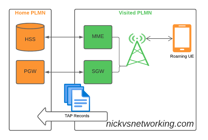
If you’ve ever worked in roaming, you’ll probably have had the misfortune of dealing with Transferred Account Procedures aka TAP files.
It’s used for billing a 2G GSM call right up to 5G data usage, if you use a service while roaming, somewhere in the world there’s a TAP file with your usage in it.
A brief history of TAP
TAP was originally specified by the GSMA in 1991 as a standard CDR interchange format between operators, for use in roaming scenarios.
Notice I said GSMA – Not 3GPP – This means there’s no 3GPP TS docs for this, it’s defined by the industry lobby group’s members, rather than the standards body.
So what does this actually mean? Well, if you’re MNO A and a customer from MNO B roams into your network, all the calls, SMS and data consumed by the roaming subscriber from MNO B will need to be billed to MNO B, by you, MNO A.
If a network operator wants to get paid for traffic used on their network by roaming subscribers, they’d better send out a TAP file to the roamer’s home network.
TAP is the file format generated my MNO A and sent to MNO B, containing all the usage charges that subscribers from MNO B have racked up while roaming into your network.
These are broken down into “Transactions” (CDRs), for events like making a call, connecting a PDN session and consuming data, or sending a text.
In the beginning of time, GSM provided only voice calling service. This meant that the only services a subscriber could consume while roaming was just making/receiving voice calls which were billed at the end of each month. – This meant billing was equally simple, every so often the visisted network would send the TAP files for the voice calls made by subscribers visited other networks, to the home networks, which would markup those charges, and add them onto the monthly invoice for each subscriber who was roaming.
But of course today, calling accounts for a tiny amount of usage on the network, but this happened gradually while passing through the introduction of SMS, CAMEL services, prepaid services, mobile data, etc. For all these services that could be offered, the TAP format had to evolve to handle each of these scenarios.
As we move towards a flat IP architecture, where voice calls and SMS sent while roaming are just data, TAP files for 4G and 5G networks only need to show data transactions, so the call objects, CAMEL parameters and SMS objects are all falling by the wayside.
What’s inside a TAP File
TAP uses the most beloved of formats – ASN1 to encode the data. This means it is strictly formatted and rigidly specified.
Each file contains a Sequence Number which is a monotonically increasing number, which allows the receiver to know if any files have been missed between the file that’s being currently parsed, an the previous file.
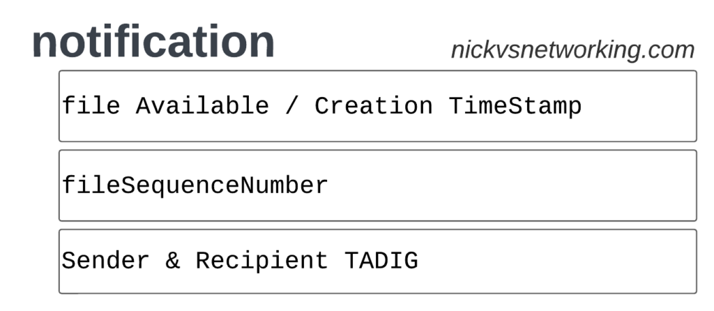
They also have a recipient and sender TADIG code, which is a code allocated by GSMA that uniquely identifies the sender and the recipient of the file.
The TAP records exist in one of two common format, Notification Records and transferBatch records.
These files are exchanged between operators, in practice this means “Dumped on an FTP server as agreed between the two”.
TAP Notification Records
Notifications are the simplest of TAP records and are used when there aren’t any CDRs for roaming events during the time period the TAP file covers.
These are essentially blank TAP files generated by the visited network to let the home network know it’s still there, but there are no roaming subs consuming services in that period.
Notification files are really simple, let’s take a look as one shown as JSON:
When we have services to bill and records to charge, that’s when instead we generate a transferBatch record.
It looks something like this:
There’s a lot going on in here, so let’s break it down section by section.
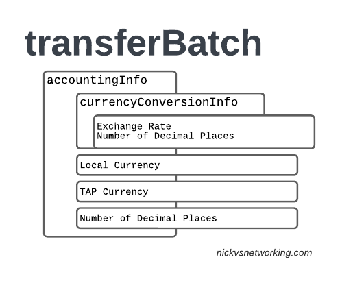
accountingInfo
The accountingInfo section specifies the currency, exchange rate parameters.
Keep in mind a TAP record generated by an operator in the US, would use USD, while the receiver of the file may be a European MNO dealing in EUR.
This gets even more complicated if you’re dealing with more obscure currencies where an intermediary currency is used, that’s where we bring in SDRs (“Special Drawing Right”) that map to the dollar value to be charged, kinda – the roaming agreement defines how many SDRs are in a dollar, in the example below we’re not using any, but you do see it.
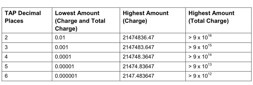
When it comes to numbers and decimal places, TAP doesn’t exactly make it easy.
Significant Digits are defined by counting the first number before the decimal point and all the numbers to the right of the decimal point, so for example the number 1.234 would be 4 significant digits (1 digit before the decimal point and 3 digits after it).
Decimal Places are not actually supported for the Value fields in the TAP file. This is tricky because especially today when roaming tariffs are quite low, these values can be quite small, and we need to represent them as an integer number. TAP defines decimal places as the number of digits after the decimal place.
When it comes to the maximum number of decimal places, this actually impacts the maximum number we can store in the field – as ASN1 strictly enforce what we put in it.
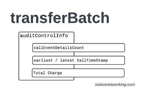
The auditControlInfo section contains the number of CDRs (callEventDetailsCount) contained in the TAP file, the timestamp of the first and last CDR in the file, the total charge and any tax charged.
All of the currency information was provided in the accountingInfo so this is just giving us our totals.
A CDR has 30 days from the time it was generated / service consumed by the roamer, to be baked into a TAP file. After this we can no longer charge for it, so it’s important that the earliestCallTimeStamp is not more than 30 days before the fileCreationTimeStamp seen in batchControlInfo.
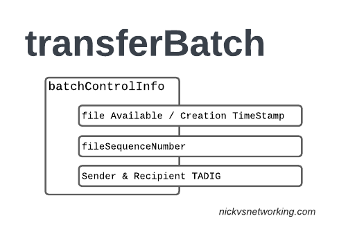
batchControlInfo
The batchControlInfo section specifies the time the TAP file became available for transfer, the time the file was created (usually the same), the sequence number and the sender / recipient TADIG codes.
As mentioned earlier, we track sequence number so the receiver can know if a TAP file has been missed; for example if you’ve got TAP file 1 and TAP file 3 comes in, you can determine you’ve missed TAP file 2.
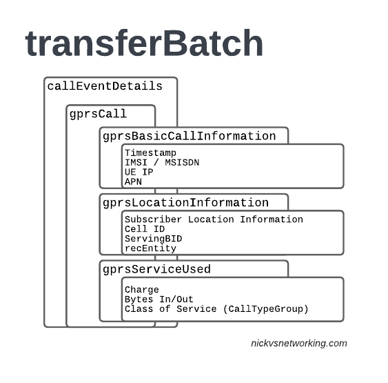
Now we’re getting to the meat & potatoes of our TAP record, the CDRs themselves.
In LTE networks these are just records of data consumption, so let’s take a look inside the gprsCall records under callEventDetails:
In the gprsBasicCallInformation we’ve got as the name suggests the basic info about the data usage event. The time when the session started, the charging ID, the IMSI and the MSISDN of the subscriber to charge, along with their IP and the APN used.
Next up we have the gprsLocationInformation – rates and tariffs may be set based on the location of the subscriber, so we need to identify the area the sub was using the services to select correct tariff / rate for traffic in this destination.
The recEntity is the index number of the SGW / PGW used for the transaction (more on that later).
Next we have the gprsServiceUsed which, again as the name suggests, details the services used and the charge.
chargeDetailList contains the charged data (Made up of dataVolumeIncoming + dataVolumeOutgoing) and the cost.
The chargeableUnits indicates the actual data consumed, however most roaming agreements will standardise on some level of rounding, for example rounding up to the nearest Kilobyte (1024 bytes), so while a sub may consume 1025 bytes of data, they’d be billed for 2045 bytes of data. The data consumed is indicated in the chargeableUnits which indicates how much data was actually consumed, before any rounding policies where applied, while the amount that is actually charged (When taking into account rounding policies) isindicated inside Charged Units.
In the example below data usage is rounded up to the nearest 1024 bytes, 134390 bytes rounds up to the nearest 1024 gives you 135168 bytes.
As this is data we’re talking bytes, but not all bytes are created equal!
VoLTE traffic, using a QCI1 bearer is more valuable than QCI 9 cat videos, and TAP records take this into account in the Call Type Groups, each of which has a different price – Call Type Level 1 indicates the type of traffic, for S8 Home Routed LTE Traffic this is 10 (HGGSN/HP-GW), while Call Type Level 2 indicates the type of traffic as mapped to QCI values:
So Call Type Level 2 set to 20 indicates that this is “20 Unspecified/default LTE QCIs”, and Call Type Level 3 can be set to any value based on a defined inter-operator tariff.
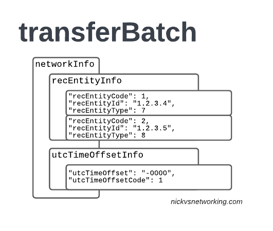
recEntityType 7 means a PGW and contains the IP of the PGW in the Home PLMN, while recEntityType 8 means SGW and is the SGW in the Visited PLMN.
So this means if we reference recEntityCode 2 in a gprsCall, that we’re referring to an SGW at 1.2.3.5.
Lastly also got the utcTimeOffsetInfo to indicate the timezones used and assign a unique code to it.
Using the Records
We as humans? These records aren’t meant for us.
They’re designed to be generated by the Visited PLMN and sent to to the home PLMN, which ingests it and pays the amount specified in the time agreed.
Generally this is an FTP server that the TAP records get dumped into, and an automated bank transfer job based on the totals for the TAP records.
Testing of the TAP records is called “TADIG Testing” and it’s something we’ll go into another day, but in essence it’s validating that the output and contents of the files meet what both operators think is the contract pricing and specifications.
So that’s it! That’s what’s in a TAP record, what it does and how we use it!
GSMA are introducing BCE – Billing & Charging Evolution, a new standard, designed to last for the next 30+ years like TAP has. It’s still in its early days, but that’s the direction the GSMA has indicated it would like to go.
Everything was working on the IMS, then I go to bed, the next morning I fire up the test device and it just won’t authenticate to the IMS – The S-CSCF generated a 401 in response to the REGISTER, but the next REGISTER wouldn’t pass.
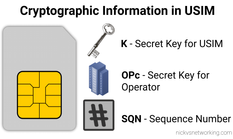
When we generate the vectors (for IMS auth and standard auth) one of the inputs to generate the vectors is the Sequence Number or SQN.
This SQN ticks over like an odometer for the number of times the SIM / HSS authentication process has been performed.
There is some leeway in the SQN – It may not always match between the SIM and the HSS and that’s to be expected. When the MME sends an Authentication-Information-Request it can ask for multiple vectors so it’s got some in reserve for the next time the subscriber attaches, and that’s allowed.
But there are limits to how far out our SQN can be, and for good reason – One of the key purposes for the SQN is to protect against replay attacks, where the same vector is replayed to the UE. So the SQN on the HSS can be ahead of the SIM (within reason), but it can’t be behind – Odometers don’t go backwards.
So the issue was with the SQN on the SIM being out of Sync with the SQN in the IMS, how do we know this is the case, and how do we fix this?
Well there is a resync mechanism so the SIM can securely tell the HSS what the current SQN it is using, so the HSS can update it’s SQN.
When verifying the AUTN, the client may detect that the sequence numbers between the client and the server have fallen out of sync. In this case, the client produces a synchronization parameter AUTS, using the shared secret K and the client sequence number SQN. The AUTS parameter is delivered to the network in the authentication response, and the authentication can be tried again based on authentication vectors generated with the synchronized sequence number.
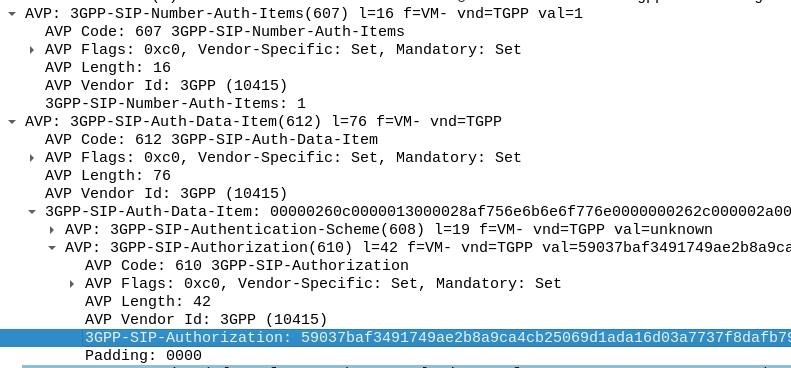
In our example we can tell the sub is out of sync as in our Multimedia Authentication Request we see the SIP-Authorization AVP, which contains the AUTS (client synchronization parameter) which the SIM generated and the UE sent back to the S-CSCF. Our HSS can use the AUTS value to determine the correct SQN.
SIP-Authorization AVP in the Multimedia Authentication Request means the SQN is out of Sync and this AVP contains the RAND and AUTN required to Resync
Note: The SIP-Authorization AVP actually contains both the RAND and the AUTN concatenated together, so in the above example the first 32 bytes are the AUTN value, and the last 32 bytes are the RAND value.
So the HSS gets the AUTS and from it is able to calculate the correct SQN to use.
Then the HSS just generates a new Multimedia Authentication Answer with a new vector using the correct SQN, sends it back to the IMS and presto, the UE can respond to the challenge normally.
Misunderstood, under appreciated and more capable than people give it credit for, is our PCRF.
But what does it do?
Most folks describe the PCRF in hand wavy-terms – “it does policy and charging” is the answer you’ll get, but that doesn’t really tell you anything.
So let’s answer it in a way that hopefully makes some practical sense, starting with the acronym “PCRF” itself, it stands for Policy and Charging Rules Function, which is kind of two functions, one for policy and one for rules, so let’s take a look at both.
Policy
In cellular world, as in law, policy is the rules.
For us some examples of policy could be a “fair use policy” to limit customer usage to acceptable levels, but it can also be promotional packages, services like “free Spotify” packages, “Voice call priority” or “unmetered access to Nick’s Blog and maximum priority” packages, can be offered to customers.
All of these are examples of policy, and to make them work we need to target which subscribers and traffic we want to apply the policy to, and then apply the policy.
Charging Rules
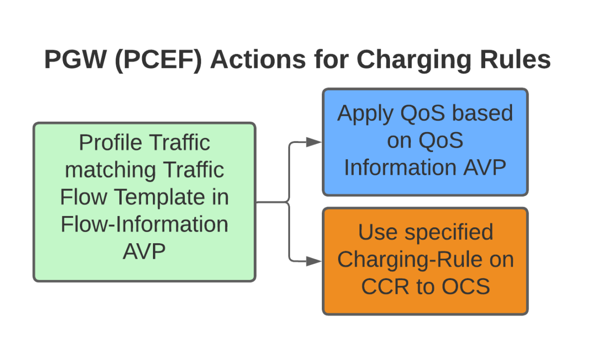
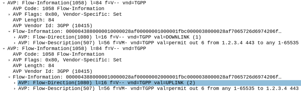
Charging Rules are where the policy actually gets applied and the magic happens.
It’s where we take our policy and turn it into actionable stuff for the cellular world.
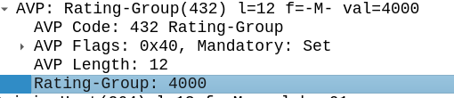
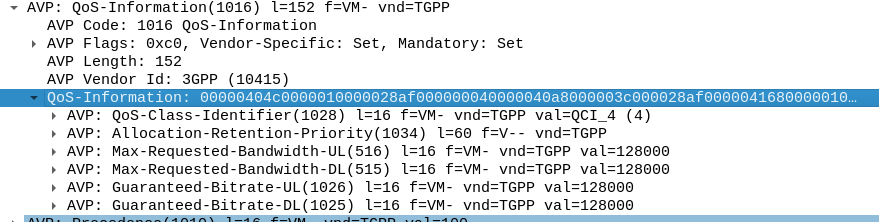
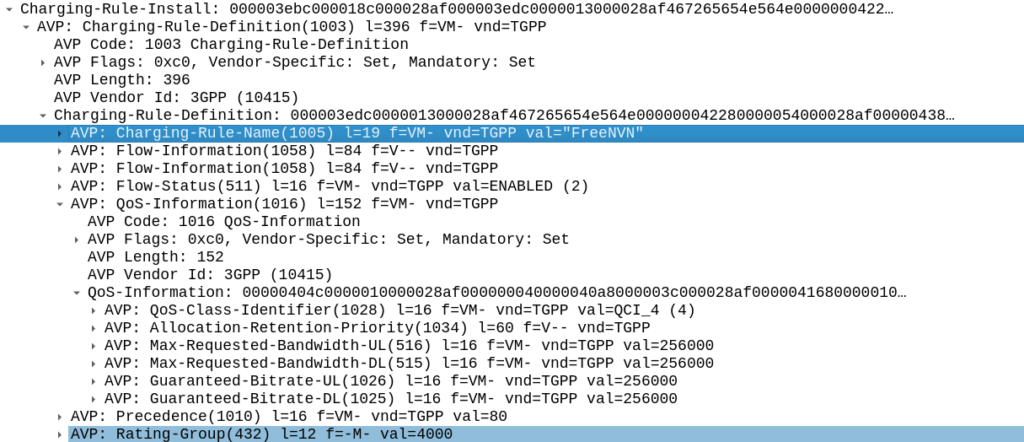
Let’s take an example of “unmetered access to Nick’s Blog and maximum priority” as something we want to offer in all our cellular plans, to provide access that doesn’t come out of your regular usage, as well as provide QCI 5 (Highest non dedicated QoS) to this traffic.
To achieve this we need to do 3 things:
Profile the traffic going to this website (so we capture this traffic and not regular other internet traffic)
Charge it differently – So it’s not coming from the subscriber’s regular balance
Up the QoS (QCI) on this traffic to ensure it’s high priority compared to the other traffic on the network
So how do we do that?
Profiling Traffic
So the first step we need to take in providing free access to this website is to filter out traffic to this website, from the traffic not going to this website.
Let’s imagine that this website is hosted on a single machine with the IP 1.2.3.4, and it serves traffic on TCP port 443. This is where IPFilterRules (aka TFTs or “Traffic Flow Templates”) and the Flow-Description AVP come into play. We’ve covered this in the past here, but let’s recap:
IPFilterRules are defined in the Diameter Base Protocol (IETF RFC 6733), where we can learn the basics of encoding them,
They take the format:
action dir proto from src to dst
The action is fairly simple, for all our Dedicated Bearer needs, and the Flow-Description AVP, the action is going to be permit. We’re not blocking here.
The direction (dir) in our case is either in or out, from the perspective of the UE.
Next up is the protocol number (proto), as defined by IANA, but chances are you’ll be using 17 (UDP) or 6 (TCP).
The from value is followed by an IP address with an optional subnet mask in CIDR format, for example from 10.45.0.0/16would match everything in the 10.45.0.0/16 network.
Following from you can also specify the port you want the rule to apply to, or, a range of ports.
Like the from, the tois encoded in the same way, with either a single IP, or a subnet, and optional ports specified.
And that’s it!
So let’s create a rule that matches all traffic to our website hosted on 1.2.3.4 TCP port 443,
permit out 6 from 1.2.3.4 443 to any 1-65535
permit out 6 from any 1-65535 to 1.2.3.4 443
All this info gets put into the Flow-Information AVPs:
With the above, any traffic going to/from 1.23.4 on port 443, will match this rule (unless there’s another rule with a higher precedence value).
Charging Actions
So with our traffic profiled, the next question is what actions are we going to take, well there’s two, we’re going to provide unmetered access to the profiled traffic, and we’re going to use QCI 4 for the traffic (because you’ll need a guaranteed bit rate bearer to access!).
Charging-Group for Profiled Traffic
To allow for Zero Rating for traffic matching this rule, we’ll need to use a different Rating Group.
Let’s imagine our default rating group for data is 10000, then any normal traffic going to the OCS will use rating group 10000, and the OCS will apply the specific rates and policies based on that.
Rating Groups are defined in the OCS, and dictate what rates get applied to what Rating Groups.
For us, our default rating group will be charged at the normal rates, but we can define a rating group value of 4000, and set the OCS to provide unlimited traffic to any Credit-Control-Requests that come in with Rating Group 4000.
This is how operators provide services like “Unlimited Facebook” for example, a Charging Rule matches the traffic to Facebook based on TFTs, and then the Rating Group is set differently to the default rating group, and the OCS just allows all traffic on that rating group, regardless of how much is consumed.
Inside our Charging-Rule-Definition, we populate the Rating-Group AVP to define what Rating Group we’re going to use.
Setting QoS for Profiled Traffic
The QoS Description AVP defines which QoS parameters (QCI / ARP / Guaranteed & Maximum Bandwidth) should be applied to the traffic that matches the rules we just defined.
As mentioned at the start, we’ll use QCI 4 for this traffic, and allocate MBR/GBR values for this traffic.
Putting it Together – The Charging Rule
So with our TFTs defined to match the traffic, our Rating Group to charge the traffic and our QoS to apply to the traffic, we’re ready to put the whole thing together.
So here it is, our “Free NVN” rule:
I’ve attached a PCAP of the flow to this post.
In our next post we’ll talk about how the PGW handles the installation of this rule.
Recently I’ve been working on open source Diameter Routing Agent implementations (See my posts on FreeDiameter).
With the hurdles to getting a DRA working with open source software covered, the next step was to get all my Diameter traffic routed via the DRAs, however I soon rediscovered a Kamailio limitation regarding support for Diameter Routing Agents.
You see, when Kamailio’s C Diameter Peer module makes a decision as to where to route a request, it looks for the active Diameter peers, and finds a peer with the suitable Vendor and Application IDs in the supported Applications for the Application needed.
Unfortunately, a DRA typically only advertises support for one application – Relay.
This means if you have everything connected via a DRA, Kamailio’s CDP module doesn’t see the Application / Vendor ID for the Diameter application on the DRA, and doesn’t route the traffic to the DRA.
The fix for this was twofold, the first step was to add some logic into Kamailio to determine if the Relay application was advertised in the Capabilities Exchange Request / Answer of the Diameter Peer.
I added the logic to do this and exposed this so you can see if the peer supports Diameter relay when you run “cdp.list_peers”.
With that out of the way, next step was to update the routing logic to not just reject the candidate peer if the Application / Vendor ID for the required application was missing, but to evaluate if the peer supports Diameter Relay, and if it does, keep it in the game.
I added this functionality, and now I’m able to use CDP Peers in Kamailio to allow my P-CSCF, S-CSCF and I-CSCF to route their traffic via a Diameter Routing Agent.