We’ve got a web based front end in our CRM which triggers Ansible Playbooks for provisioning of customer services, this works really well, except I’d been facing a totally baffling issue of late.
Ansible Plays (Provisioning jobs) would have variables set that they inherited from other Ansible Plays, essentially if I set a variable in Play X and then ran Play Y, the variable would still be set.
I thought this was an issue with our database caching the play data showing the results from a previous play, that wasn’t the case.
Then I thought our API that triggers this might be passing extra variables in that it had cached, wasn’t the case.
In the end I ran the Ansible function call in it’s simplest possible form, with no API, no database, nothing but plain vanilla Ansible called from Python
    # Run the actual playbook
    r = ansible_runner.run(
        private_data_dir='/tmp/',
        playbook=playbook_path,
        extravars=extra_vars,
        inventory=inventory_path,
        event_handler=event_handler_obj.event_handler,
        quiet=False
    )
And I still I had the same issue of variables being inherited.
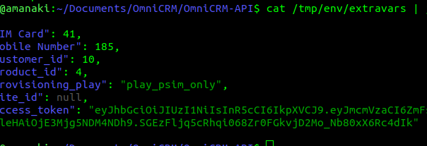
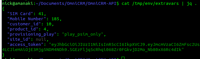
So what was the issue? Well the title gives it away, the private_data_dir parameter creates a folder in that directory, called env/extravars which a JSON file lives with all the vars from all the provisioning runs.
Removing the parameter from the Python function call resolved my issue, but did not give me back the half a day I spent debugging this…
This is the next post in my series on SS7, and today we’re taking a look at SCCP the Signalling Connection Control Part (SCCP).
High Level
Global Title uses the routing features from SCCP, which is another layer on top of MTP3.
SCCP allows us to route on more than just point code, instead we can route based on two new fields, Subsystem Number and Global Title.
Subsystem Number is the type of system we are looking to reach, ie an HLR, MSC, CAMEL Gateway, etc.
The Global Title generally looks like an E.164 formatted phone number, and often it is just that.
Somewhere along the chain (typically at the end of it) an STP somewhere needs to perform Global Title Translation to analyse the SCCP header (Subsystem Number, Point Code & Global Title) and finally turn that into a single point code to route the MTP3 message to.
The advantage of this is we are no longer just limited to routing messages based on Point Code.
This is how the international SS7 Network used for roaming is structured and addressed – All using Global Title rather than Point Codes.
The need for SCCP
For starters, after all this talk of MTP3 and Point Codes, why the need to add SCCP?
Let’s go back in time and look at the motivators…
1. Address space is finite
Point codes are great, and when we’ve spoken about them before, I’ve compared them to IPv4 address, but rather than ranging from 0.0.0.0 to 255.255.255.255 (32 bits on IPv4) international signaling point codes range from 0.0.0 to 7.255.7 (14 bits).
The problem with IPv4’s 32 bit addresses is they run out. The problem with the ITU International Signaling Point Codes is that they too, are a limited resource with only 16,383 possible ISPCs.
~700 operators worldwide each with ~100 network elements would be 70k point codes to address them all – That’s not going to fit into our 16k possible Point Codes.
Global Title fixes this, because we’re able to use E.164 phone number ranges (which are plentiful) for addressing, we’re still not at IPv6 levels of address space, but pretty hefty.
2. Service Discovery by Subsystem
Now imagine you’re a VLR looking to find an HLR. The VLR and the HLR are both connected to an STP, but how does the VLR know where to reach the HLR?
One option would be to statically set every route for the Point Code of every HLR into every possible VLR and visa-versa, but that gets messy fast.
What if the VLR could just send a request to the STP and indicate that the request needs to be routed to any HLR, and the STP takes care of finding a SS7 node capable of handling the request, much a Diameter Routing Agent routes based on Application ID.
SCCP’s “Subsystem Number” routing can handle this as we can route based on SSN.
3. Service Discovery by MSISDN
Having an SMS destined to a given MSISDN requires the SMSc to know where to route it.
Likewise an MSC wanting to call a given number.
There’s a lot of MSISDN ranges. Like a lot. Like every phone mobile number.
Having every a table on every SSP/SCP in the network know where every MSISDN range is in the world and what point code to go through to reach it is not practical.
Instead, being able to have the SCP/SSPs (like our MSC or SMSc) send all off-net traffic to an STP frees us the individual SCP/SSPs from this role; they just forward it to their connected STP.
Our STP can analyse the destination MSISDN and make these routing decisions for us, using Global Title Translation based on rules in the Global Title Table on the STP.
For example by adding each of the domestic / national MSISDN ranges/prefixes into the Global Title Table on the STP (along with the corresponding point code to route each one to), the STP can look at the destination MSISDN in the message and forward to the STP for the correct operator.
Likewise a route can match anything where the Global Title address is outside of the local country and send it to an international signaling provider.
Global title takes care of this as we can route based on a phone number.
4. Tokenistic Security
By “Hiding” network elements behind Global Titles, you don’t expose as much information about your internal network, and the only way people can “find” your network elements would be scanning through all the possible addresses in your (publicly advertised) Global Title range (wardialing is back baby!).
But the phrases “Security” and “SS7” don’t really belong together…
The SCCP Header
The SCCP header has a Called Party and a Calling Party, and this is where the magic happens.
These can be made up for any number of 3 parts:
Global Title Address
Subsystem Number
Point Code
We can route on any combination of these.
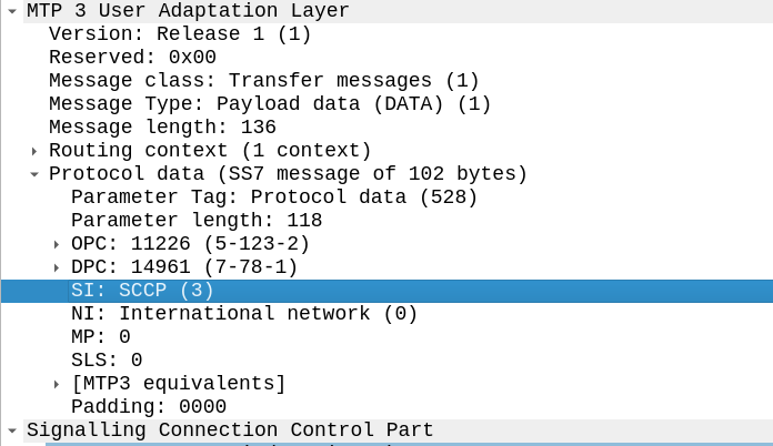
To indicate we’re using SCCP, we set the Signaling Indicator bit in the M3UA / MTP3 message to SCCP:
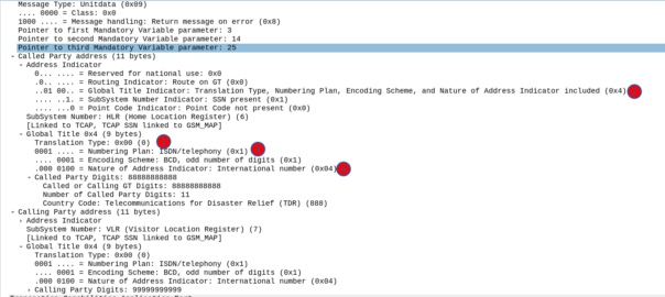
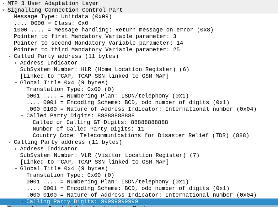
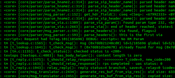
Great, now we can look at our SCCP header.
It looks like there’s a lot going on, but we can see the calling and called party (888888888 is called by 9999999999) with the Subsystem number set (888888888 is called for subsystem HLR, from 999999999 which is a VLR).
The closest TCP/IP analogy I can think of here is that of port numbers, there’s still an IP (Point code) but the port number allows us to specify multiple applications that run at a higher layer. This analogy falls down when we consider that the Point Code is generally set to that of your STP, not the final STP.
For this to work, we’ve got to have at least one Signaling Transfer Point in the flow, where we send the request to.
Somewhere (generally at the end of the chain of STPs), an STP is going to perform Global Title Translation.
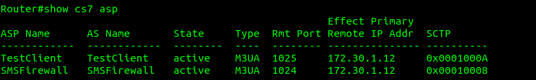
What does this look like? Well let’s have a look at my GT table for the example above, in my lab network, I’ve got two nodes attached (via M3UA but could equally be on MTP3 links), my test MAP client where I’m originating this traffic, and an SMS Firewall, I can see they’re both up here:
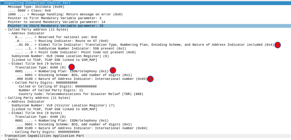
Now knowing this I need to setup my SCCP routing for Global Title. In the screenshot above, the Called Party was 888888888 with Subsystem Number 7. Inside the SCCP request, there’s a few other fields, the Translation Type we have set to 0, Global Title Indicator is 4 (route on Global Title), while Numbering Plan Indicator is 1 (ISDN) and Nature of Address Indicator is 4 (International).
So on my Cisco ITP I define a GTT Selector to target traffic with these values, Translation Type is 0, Global Title Indicator is 4, Number Plan is 1 and the Nature of Address Indicator is 4.
So we’d define a Global Title Translation selector like the one below to match this traffic:
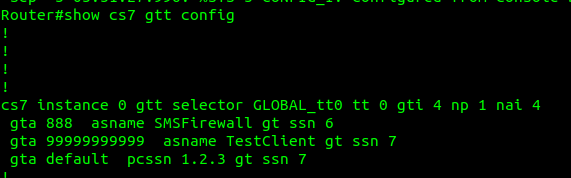
But that’s only matching the group of traffic, it’s not going to match based on the actual SCCP Called Party. So now I need to define a translation for each Global Title address (Called /Calling party) or prefix I want to route, I’ve setup anything starting with 888 to route to the `SMSFirewall` ASP endpoint.
I could stop here and my request addressed to 888888888 would make it to the SMSFirewall ASP, but the response never would, like in all SS7 routing, we need to define the return route translation too, which is what I’ve done for 999999 to route to the TestClient.
Lastly I’ve added a wildcard route, this means if this STP doesn’t know how to resolve a GT address matching the rules in the top line, it’ll forward the request to the STP at point code 1.2.3 – This is how you’d do your connection to an IPX / Signaling exchange.
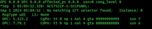
Debugging this can be a massive pain in the backside, but if you enable logging you can see when GT rules are not matched, like in the example below.
If your network is quiet enough, it’s sometimes easier to just make your rules based on what you observe failing to route.
So with those routes in place, when we send a request with the Global Title called party starting with 8888888 it’s routed to M3UA ASP SMSFirewall, which handles the request, and then sends the response back to the MAPClient M3UA ASP.
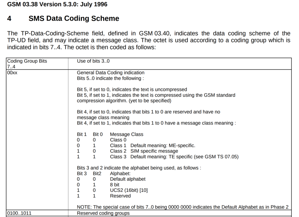
The Data Coding Scheme (DCS or TP-DCS) header in an SMS body indicates what encoding is used in that message.
It means if we’re using UCS-2 (UTF16) special characters like Emojis etc, in in our message, the phone knows to decode the data in the message body using UTF, because the Data Coding Scheme (DCS) header indicates the contents are encoded in UTF.
Likewise, if we’re not using any fancy characters in our message and the message is encoded as plain old GSM7, we set set the DCS to 0 to indicate this is using GSM7.
From my experience, I’d always assumed that DCS0 (Default) == GSM7, but today I learned, that’s not always the case. Some SMSc entities treat DCS0 as Latin.
Let me explain why this is stupid and why I wasted a lot of time on this.
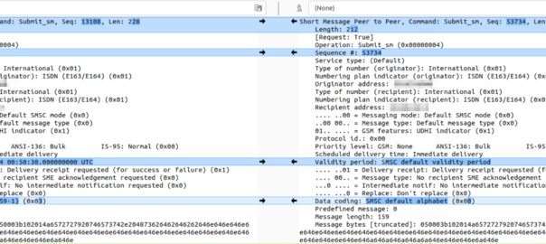
We can indicate that a message is encoded as Latin by setting the DCS to 0x03:
We cannot indicate that the message is encoded as GSM7 through anything other than the default alphabet (DCS 0).
Latin has it’s own encoding flag, if I wanted the message treated as Latin, I’d indicate the message encoding is Latin in the DCS bit!
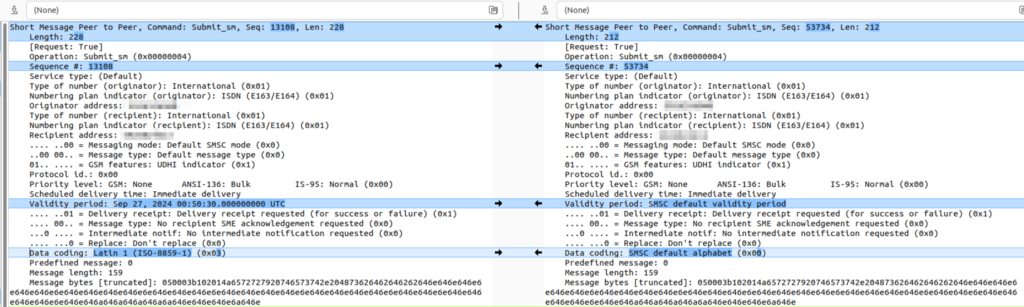
I spent a bunch of time trying to work out why a customer was having issues getting messages to subscribers on another operator, and it turned out the other operator treats messages we send to them on SMPP with DCS0 as Latin encoding, and then cracks the sads when trying to deliver it.
The above diff shows the message we send (Right), and the message they dry to deliver (left).
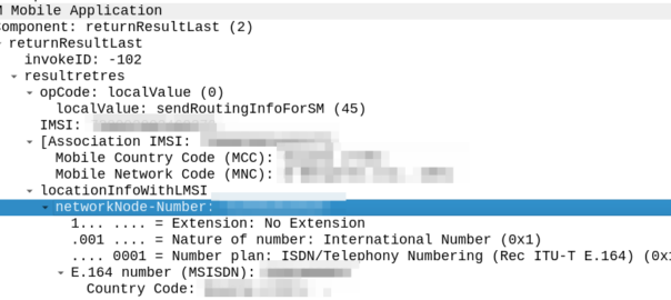
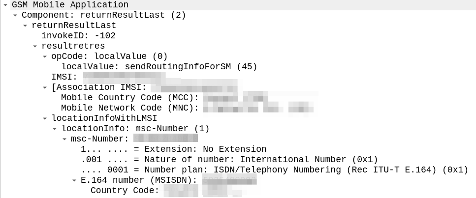
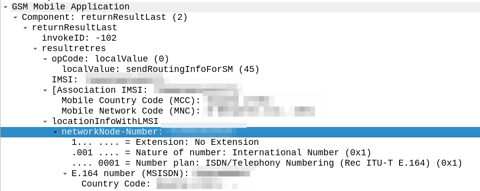
The other day I was facing an issue with our SMSc inter-working with another operator via MAP.
Our SRI-for-SM responses were relayed back to their nodes, but it was like it couldn’t parse the message.
I got some “known good” traffic to compare this against to work out what we’re doing wrong.
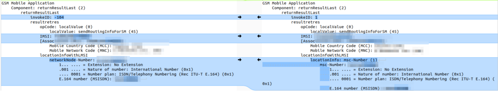
The difference in the two examples below is subtle, but it’s there – On the example on the left (failing) we are including an msc-number in the locationInfoWithLMSI field, while on the right we’ve got a “Network Node Number”.
“Okay” I thought to myself, we’re just doing something wrong with the encoding of the MAP body, so I did my usual diff trick from Wireshark:
Oddly in the raw form both these values decode the same, if I feed the values on the left into our decoder, and then encode, I get the values on the right, with the exact same hex body – and this is all ASN.1; so there’s very little room for error anyway.
So what gives? Why does Wireshark show one MAP body differently to the other, with the same hex bytes?
Well, the issue is not within my GSM MAP body and the content I include there, but rather in the TCAP layer above it, specifically the `application-context-name`.
We’re indicating support for GSM MAP v3 (0.4.0.0.1.0.20.3), while the other operator is using MAPv2 ( 0.4.0.0.1.0.20.2 ) even though their IR.21 indicates it should be GSM MAP v3.
Now our SRI-for-SM responses are based on the GSM MAP version received, rather than reported as supported, and we don’t have to deal with this for handling requests anymore.
And bam, now when we run Kamailio we’ll get all the logic that rtpengine exposes when being called.
By setting cfgtrace we can enable a config trace as well, and as we step through our Kamailio config file for a SIP message, we can see what’s going on at every step.
So if you’re like me, you can use the debugger module, combined with reading through the source code, to prove every singletime that the issue is with my not understanding the function properly, and never the logic of the Kamailio module!
Technology is constantly evolving, new research papers are published every day.
But recently I was shocked to discover I’d missed a critical development in communications, that upended Shannon’s “A mathematical theory of communication”.
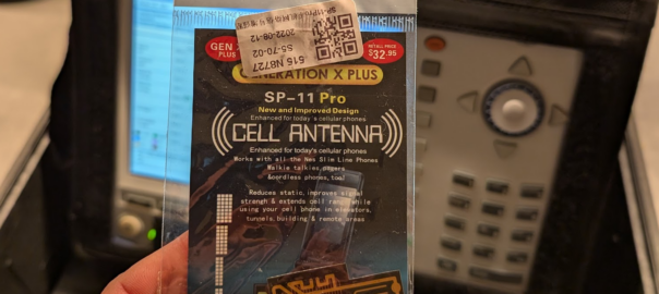
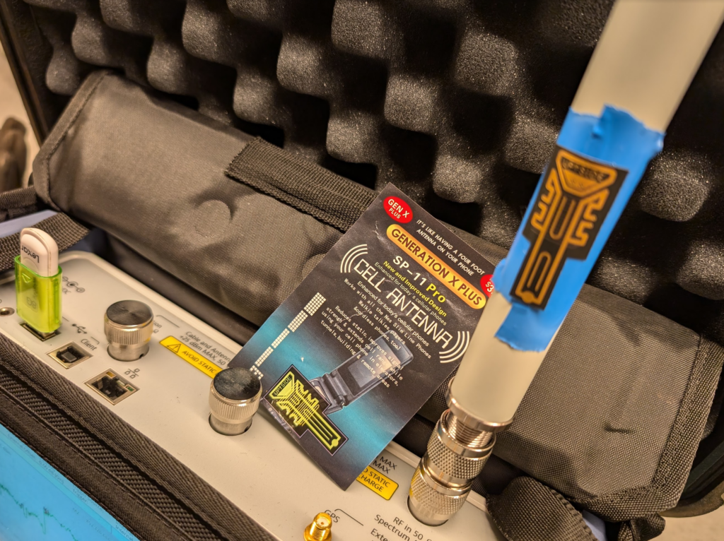
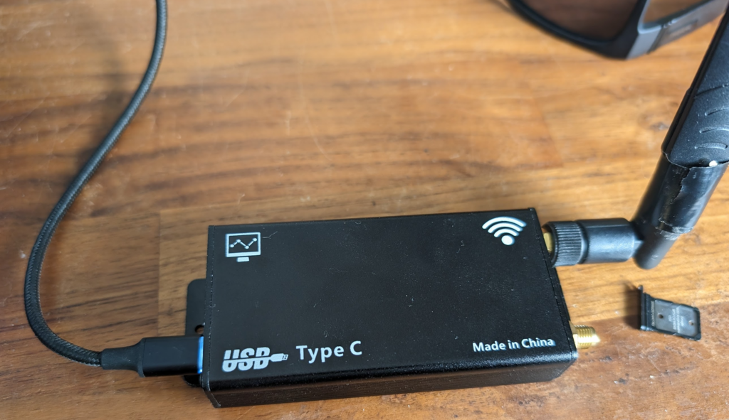
I’m talking of course, about the GENERATION X PLUS SP-11 PRO CELL ANTENNA.
I’ve been doing telecom work for a long time, while I mostly write here about Core & IMS, I am a licenced rigger, I’ve bolted a few things to towers and built my fair share of mobile coverage over the years, which is why I found this development so astounding.
With this, existing antennas can be extended, mobile phone antennas, walkie talkies and cordless phones can all benefit from the improvement of this small adhesive sticker, which is “Like having a four foot antenna on your phone”.
So for the bargain price of $32.95 (Or $2 on AliExpress) I secured myself this amazing technology and couldn’t wait to quantify it’s performance.
Think of the applications – We could put these stickers on 6 ft panel antennas and they’d become 10ft panels. This would have a huge effect on new site builds, minimize wind loading, less need for tower strengthening, more room for collocation on the towers due to smaller equipment footprint.
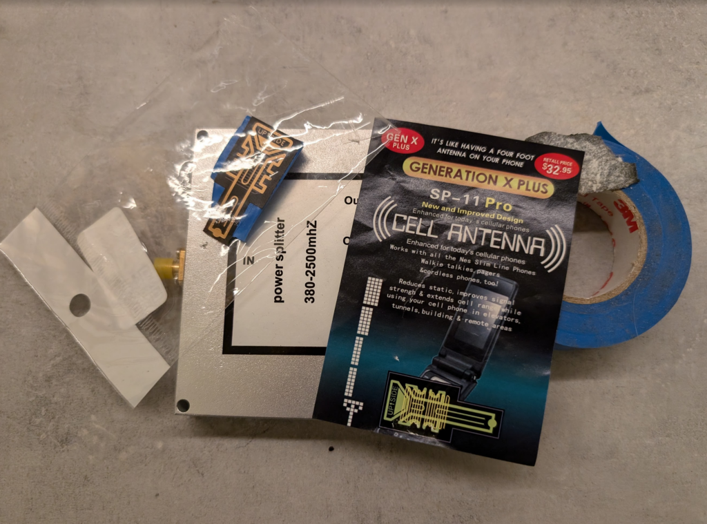
Luckily I have access to some fancy test equipment to really understand exactly how revolutionary this is.
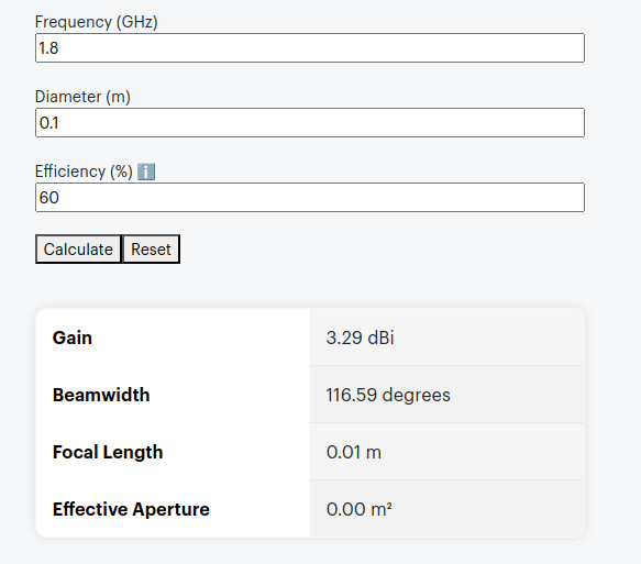
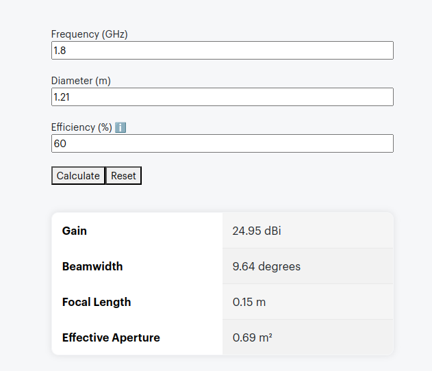
The packaging says it’s like having a 4 foot antenna on your phone, let’s do some very simple calculations, let’s assume the antenna in the phone is currently 10cm, and that with this it will improve to be 121cm (four feet).
Projected Gain (Post Sticker)Formulas Used
According to some basic projections we should see ~21dB gain by adding the sticker, that’s a 146x increase in performance!
Man am I excited to see this in action.
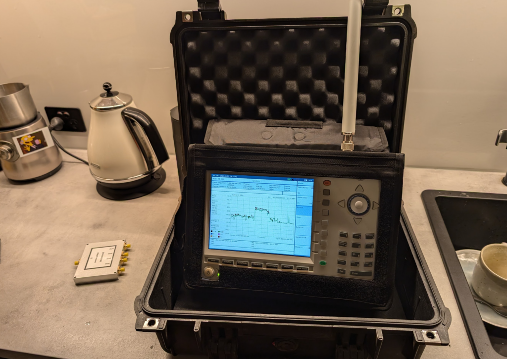
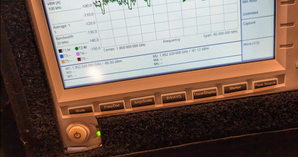
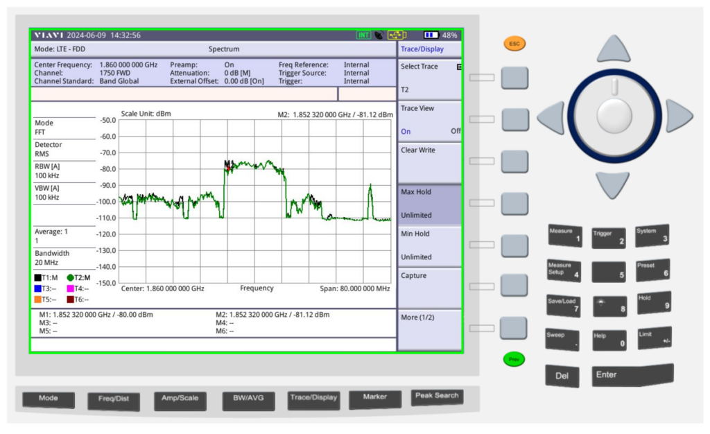
Fortunately I have access to some fun cellular test equipment, including the Viavi CellAdvisor and an environmentally controlled lab my kitchen bench.
I put up a 1800Mhz (band 3) LTE carrier in my office in the other room as a reference and placed the test equipment into the test jig (between the sink and the kettle).
We then took baseline readings from the omni shown in the pictures, to get a reading on the power levels before adding the sticker.
We are reading exactly -80dBm without the sticker in place, so we expertly put some masking tape on the omni (so we could peel it off) and applied the sticker antenna to the tape on the omni antenna.
At -80dBm before, by adding the 21dB of gain, we should be put just under -60dBm, these Viavi units are solid, but I was fearful of potentially overloading the receive end from the gain, after a long discussion we agreed at these levels it was unlikely to blow the unit, so no in-line attenuation was used.
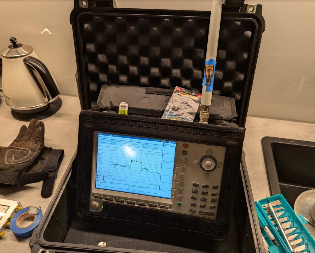
Okay, </sarcasm> I was genuinely a little surprised by what we found; there was some gain, as shown in the screenshot below.
Marker 1 was our reference without the sticker, while reference 2 was our marker with the sticker, that’s a 1.12dB gain with the sticker in place. In linear terms that’s a ~30% increase in signal strength.
Screenshot
So does this magic sticker work? Well, kinda, in as much that holding onto the Omni changes the characteristics, as would wrapping a few turns of wire around it, putting it in the kettle or wrapping it in aluminum foil. Anything you do to an antenna to change it is going to cause minor changes in characteristic behavior, and generally if you’re getting better at one frequency, you get worse at another, so the small gain on band 3 may also lead to a small loss on band 1, or something similar.
So what to make of all this? Maybe this difference is an artifact from moving the unit to make a cup of tea, the tape we applied or just a jump in the LTE carrier, or maybe the performance of this sticker is amazing after all…
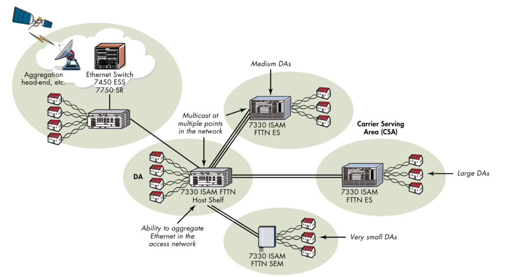
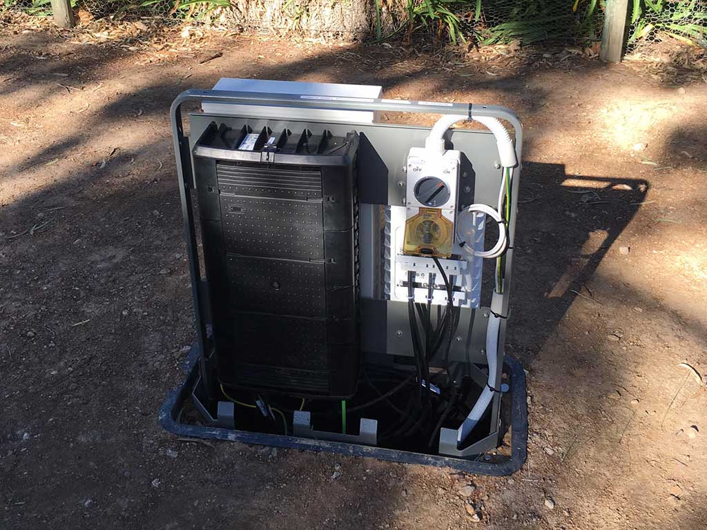
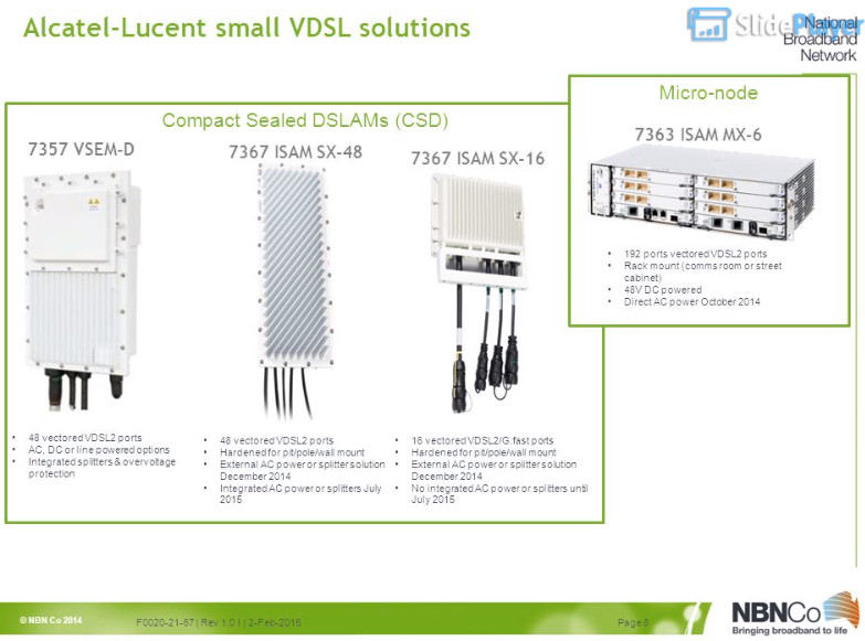
We’ve covered most of the types of NBN Node, but the “Micronode” isn’t something we’ve looked at. Micronodes are “satellites” that hang off a larger Nokia ISAM and act as NBN FTTN DSLAMs.
In NBN documentation these are referred to as “Compact Sealed DSLAMs” or CSDs, and in Nokia/Alcatel documentation these are called Sealed Expansion Modules (SEMs) – Regardless of what you call them, they act as 48 port VDSL capable DSLAMs like rest of the Nokia / Alcatel ISAM family that are used for FTTN.
They are similar in concept to the NBN FTTC program, except these units are not reverse powered, and they have a higher subscriber count.
They’re housed in the green cabinets that were used for the HFC / Pay TV networks installed in some locations underground.
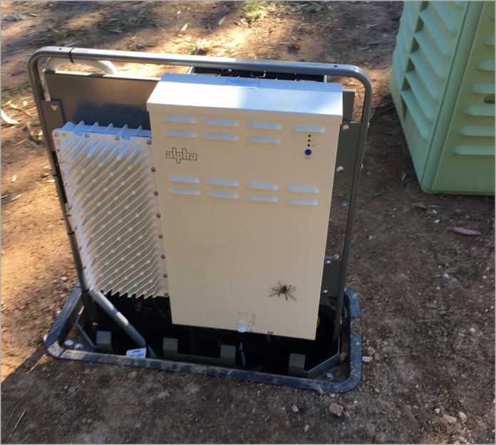
The CSD are a Nokia 7367 ISAM SX-48V (White box with the heat sink on the left of the photo below) which is connected directly back to the nearest exchange.
There is also an internal PSU with batteries powered from the incoming unmetered AC supply and a PSU is supplied by Alpha technologies in the photo on the right (With the spider).
On the flip side of the unit is where the copper pairs come in, and the DSLAM X-Pairs go out, and a small fibre splice tray.
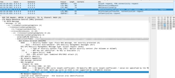
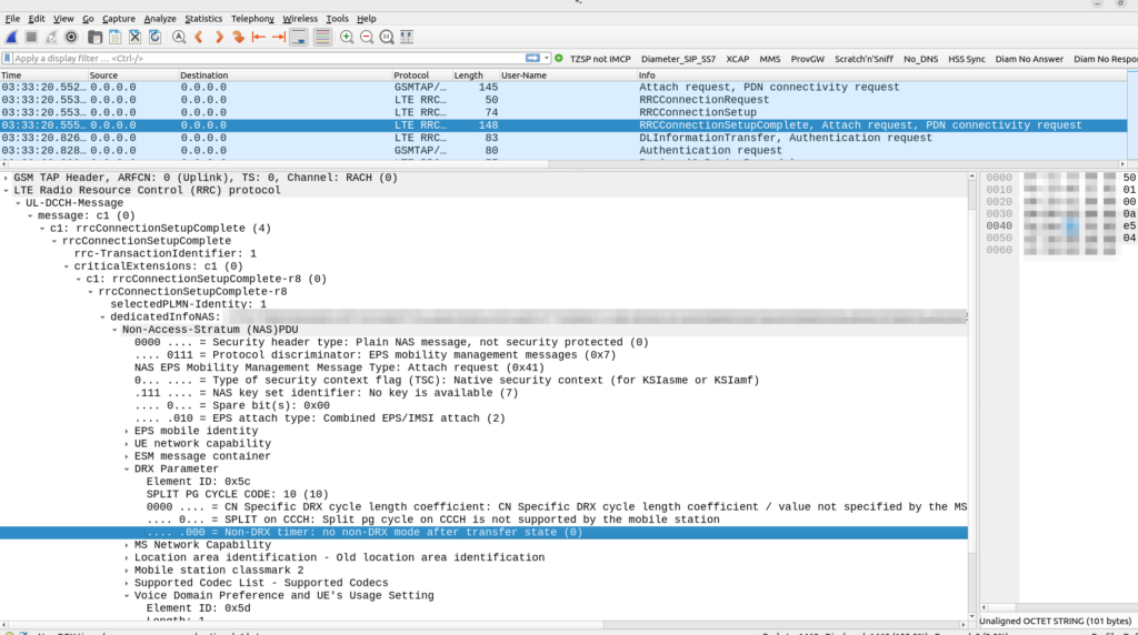
Recently we were on a project and our RAN guy was seeing UEs hand between one layer and another over and over. The hysteresis and handover parameters seemed correct, but we needed a way to see what was going on, what the eNB was actually advertising and what the UE was sending back.
In a past life I had access to expensive complicated dedicated tooling that could view this information transmitted by the eNB, but now, all I need is a cellphone or a modem with a Qualcomm chip.
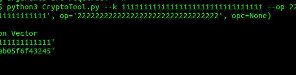
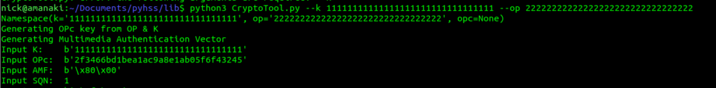
Namespace(k='11111111111111111111111111111111', op='22222222222222222222222222222222', opc=None) Generating OPc key from OP & K Generating Multimedia Authentication Vector Input K: b'11111111111111111111111111111111' Input OPc: b'2f3466bd1bea1ac9a8e1ab05f6f43245' Input AMF: b'\x80\x00'
Of course, being open source, you can grab the functions out of this and make a little script to convert everything in a CSV or whatever format your key data is in.
So what about OPc to OP? Well, this is a one-way transaction, we can’t get the OP Key from an OPc & Ki.
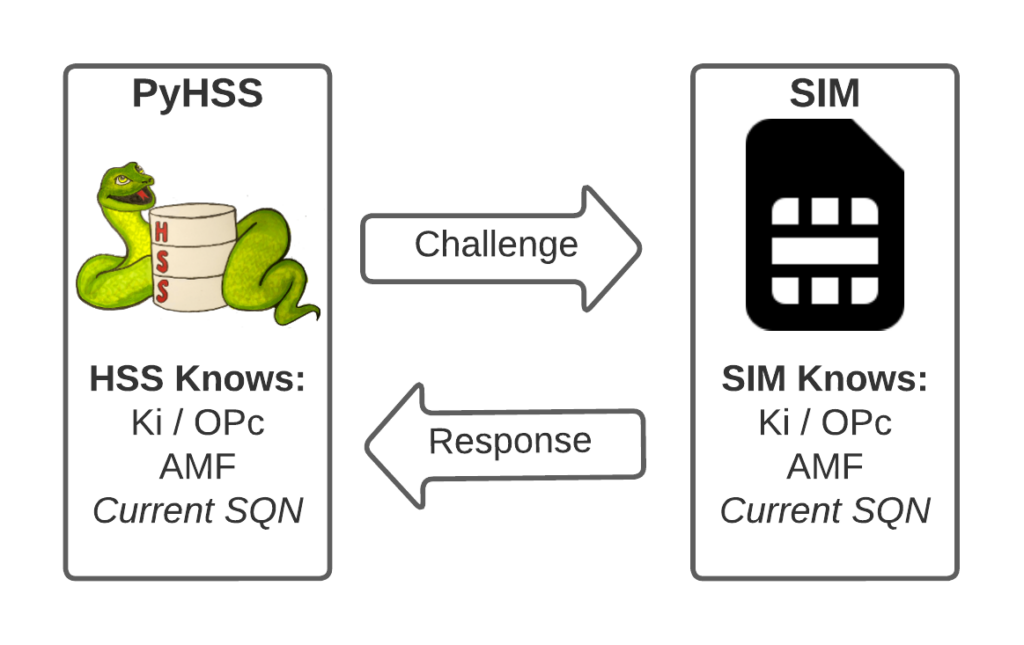
I’ve written about Milenage and SIM based security in the past on this blog, and the component that prevents replay attacks in cellular network authentication is the Sequence Number (Aka SQN) stored on the SIM.
Think of the SQN as an incrementing odometer of authentication vectors. Odometers can go forward, but never backwards. So if a challenge comes in with an SQN behind the odometer (a lower number), it’s no good.
Why the SQN is important for Milenage Security
Every time the SIM authenticates it ticks up the SQN value, and when authenticating it checks the challenge from the network doesn’t have an SQN that’s behind (lower than) the SQN on the SIM.
Let’s take a practical example of this:
The HSS in the network has SQN for the SIM as 8232, and generates an authentication challenge vector for the SIM which includes the SQN of 8232. The SIM receives this challenge, and makes sure that the SQN in the SIM, is equal to or less than 8232. If the authentication passes, the new SQN stored in the SIM is equal to 8232 + 1, as that’s the next valid SQN we’d be expecting, and the HSS incriments the counters it has in the same way.
By constantly increasing the SQN and not allowing it to go backwards, means that even if we pre-generated a valid authentication vector for the SIM, it’d only be valid for as long as the SQN hasn’t been authenticated on the SIM by another authentication request.
Imagine for example that I get sneaky access to an operator’s HSS/AuC, I could get it to generate a stack of authentication challenges that I could use for my nefarious moustache-twirling purposes whenever I wanted.
This attack would work, but this all comes crumbling down if the SIM was to attach to the real network after I’ve generated my stack of authentication challenges.
If the SQN on the SIM passes where it was when the vectors were generated, those vectors would become unusable.
It’s worth pointing out, that it’s not just evil purposes that lead your SQN to get out of Sync; this happens when you’ve got subscriber data split across multiple HSSes for example, and there’s a mechanism to securely catch the HSS’s SQN counter up with the SQN counter in the SIM, without exposing any secrets, but it just ticks the HSS’s SQN up – It never rolls back the SQN in the SIM.
The Flaw – Draining the Pool
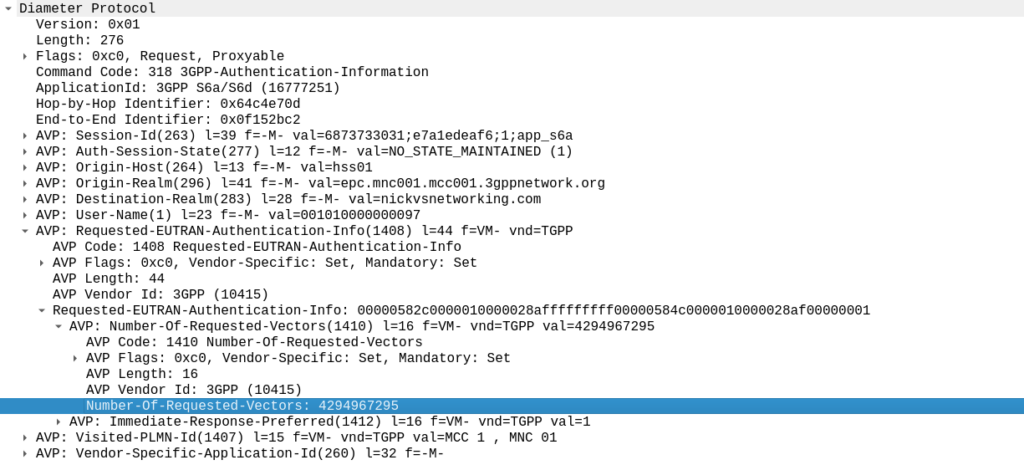
The Authentication Information Request is used by a cellular network to authenticate a subscriber, and the Authentication Information Answer is sent back by the HSS containing the challenges (vectors).
When we send this request, we can specify how many authentication challenges (vectors) we want the HSS to generate for us, so how many vectors can you generate?
TS 129 272 says the Number-of-Requested-Vectors AVP is an Unsigned32, which gives us a possible pool of 4,294,967,295 combinations. This means it would be legal / valid to send an Authentication Information Request asking for 4.2 billion vectors.
It’s worth noting that that won’t give us the whole pool.
Sequence numbers (SQN) shall have a length of 48 bits.
TS 133 102
While the SQN in the SIM is 48 bits, that gives us a maximum number of values before we “tick over” the odometer of 281,474,976,710,656.
If we were to send 65,536 Authentication-Information-Requests asking for 4,294,967,295 a piece, we’d have got enough vectors to serve the sub for life.
Except the standard allows for an unlimited number of vectors to be requested, this would allow us to “drain the pool” from an HSS to allow every combination of SQN to be captured, to provide a high degree of certainty that the SQN provided to a SIM is far enough ahead of the current SQN that the SIM does not reject the challenges.
Can we do this?
Our lab has access to HSSes from several major vendors of HSS.
Out of the gate, the Oracle HSS does not allow more than 32 vectors to be requested at the same time, so props to them, but the same is not true of the others, all from major HSS vendors (I won’t name them publicly here).
For the other 3 HSSes we tried from big vendors, all eventually timed out when asking for 4.2 billion vectors (don’t know why that would be *shrug*) from these HSSes, it didn’t get rejected.
This is a lab so monitoring isn’t great but I did see a CPU spike on at least one of the HSSes which suggests maybe it was actually trying to generate this.
Of course, we’ve got PyHSS, the greatest open source HSS out there, and how did this handle the request?
Well, being standards compliant, it did what it was asked – I tested with 1024 vectors I’ll admit, on my little laptop it did take a while. But lo, it worked, spewing forth 1024 vectors to use.
So with that working, I tried with 4,294,967,295…
And I waited. And waited.
And after pegging my CPU for a good while, I had to get back to real life work, and killed the request on the HSS.
In part there’s the fact that PyHSS writes back to a database for each time the SQN is incremented, which is costly in terms of resources, but also that generating Milenage vectors in LTE is doing some pretty heavy cryptographic lifting.
The Risk
Dumping a complete set of vectors with every possible SQN would allow an attacker to spoof base stations, and the subscriber would attach without issue.
Historically this has been very difficult to do for LTE, due to the mutual network authentication, however this would be bypassed in this scenario.
The UE would try for a resync if the SQN is too far forward, which mitigates this somewhat.
Cryptographically, I don’t know enough about the Milenage auth to know if a complete set of possible vectors would widen the attack surface to try and learn something about the keys.
Mitigations / Protections
So how can operators protect ourselves against this kind of attack?
Different commercial HSS vendors handle this differently, Oracle limits this to 32 vectors, and that’s what I’ve updated PyHSS to do, but another big HSS vendor (who I won’t publicly shame) accepts the full 4294967295 vectors, and it crashes that thread, or at least times it out after a period.
If you’ve got a decent Diameter Routing Agent in place you can set your DRA to check to see if someone is using this exploit against your network, and to rewrite the number of requested vectors to a lower number, alert you, or drop the request entirely.
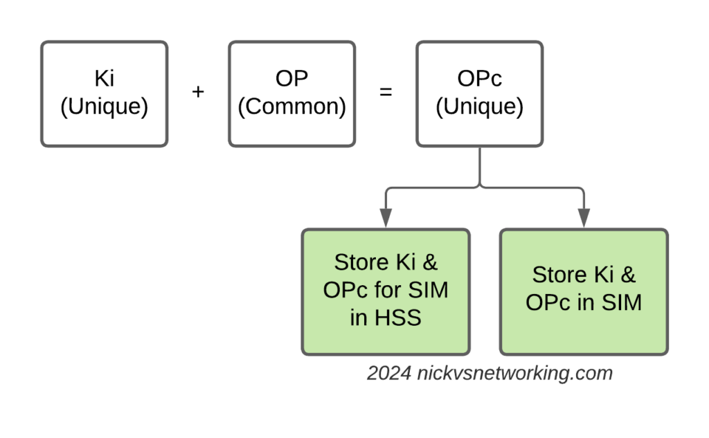
Having common OP keys is dumb, and I advocate to all our operator customers to use OP keys that are unique to each SIM, and use the OPc key derived anyway. This means if one SIM spilled it’s keys, the blast doesn’t extend beyond that card.
In the long term, it’d be good to see 3GPP limit the practical size of the Number-of-Requested-Vectors AVP.
2G/3G Impact
Full disclosure – I don’t really work with 2G/3G stacks much these days, and have not tested this.
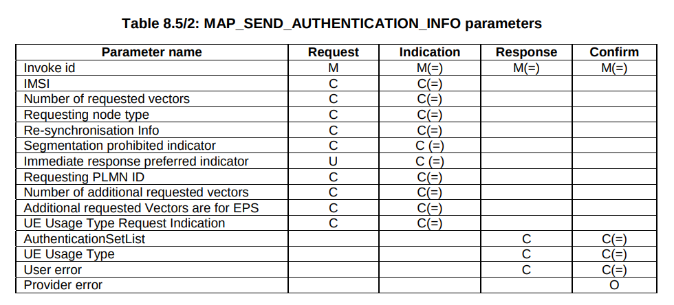
MAP is generally pretty bandwidth constrained, and to transfer 280 billion vectors might raise some eyebrows, burn out some STPs and take a long time…
But our “Send Authentication Info” message functions much the same as the Authentication Information Request in Diameter, 3GPP TS 29.002 shows we can set the number of vectors we want:
5GC Vulnerability
This only impacts LTE and 5G NSA subscribers.
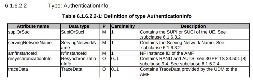
TS 29.509 outlines the schema for the Nausf reference point, used for requesting vectors, and there is no option to request multiple vectors.
Summary
If you’ve got baddies with access to your HSS / HLR, you’ve got some problems.
But, with enough time, your pool could get drained for one subscriber at a time.
This isn’t going to get the master OP Key or plaintext Ki values, but this could potentially weaken the Milenage security of your system.
One of the new features of 5GC is the introduction of Service Based Interfaces (SBI) which is part of 5GC’s Service Based Architecture (SBA).
Let’s start with the description from the specs:
3GPP TS 23.501 [3] defines the 5G System Architecture as a Service Based Architecture, i.e. a system architecture in which the system functionality is achieved by a set of NFs providing services to other authorized NFs to access their services.
3GPP TS 29.500 – 4.1 NF Services
For that we have two key concepts, service discovery, and service consumption
Services Consumer / Producers
That’s some nice words, but let’s break down what this actually means, for starters, let’s talk about services.
In previous generations of core network we had interfaces instead of services. Interfaces were the reference point between two network elements, describing how the two would talk. The interfaces were the protocols the two interfaces used to communicate.
For example, in EPC / LTE S6a is the interface between the MME and the HSS, S5 is the interface between the S-GW and P-GW. You could lookup the 3GPP spec for each interface to understand exactly how it works, or decode it in Wireshark to see it in action.
5GC moves from interfaces to services. Interfaces are strictly between two network elements, the S6a interface is only used between the MME and the HSS, while a service is designed to be reusable.
This means the Service Based Interface N5g-eir can be used by the AMF, but it could equally be used by anyone else who wants access to that information.
3GPP defines the service in the form of service producer (The EIR produces the N5g-eir service) and the service consumer (The client connecting to the N5g-eir service), but doens’t restrict which network elements can
This gets away from the soup of interfaces available, and instead just defines the services being offered, rather than locking the
“service consumers” (which can be thought of clients in a client/server model) can discover “service producers” (like servers in a client/server model).
Our AMF, which acts as a “service consumer” consuming services from the UDM/UDR and SMF.
Service Discovery – Automated Discovery of NF Services
Service-Based Architecture enables 5G Core Network Function service discovery.
In simple terms, this means rather that your MME being told about your SGW, the nodes all talk to a “Network Repository Function” that returns a list of available nodes.
The mobility management and connection management process in 5GC focuses on Connection Management (CM) and Registration Management (RM).
Registration Management (RM)
The Registration Management state (RM) of a UE can either be RM-Registered or RM-Deregistered. This is akin to the EMM state used in LTE.
RM-Deregistered Mode
From the Core Network’s perspective (Our AMF) a UE that is in RM-Deregistered state has no valid location information in the AMF for that UE. The AMF can’t page it, it doesn’t know where the UE is or if it’s even turned on.
From the UE’s perspective, being in RM-Deregistered state could mean one of a few things:
UE is in an area without coverage
UE is turned off
SIM Card in the UE is not permitted to access the network
In short, RM-Deregistered means the UE cannot be reached, and cannot get any services.
RM-Registered Mode
From the Core Network’s perspective (the AMF) a UE in RM-Registered state has sucesfully registered onto the network.
The UE can perform tracking area updates, period registration updates and registration updates.
There is a location stored in the AMF for the UE (The AMF knows at least down to a Tracking Area Code/List level where the UE is).
The UE can request services.
Connection Management (CM)
Connection Management (CM) focuses on the NAS signaling connection between the UE and the AMF.
To have a Connection Management state, the Registration Management procedure must have successfully completed (the UE being in RM-Registered) state.
A UE in CM-Connected state has an active signaling connection on the N1 interface between the UE and the AMF.
CM-Idle Mode
In CM-Idle mode the UE has no active NAS connection to the AMF.
UEs typically enter this state when they have no data to send / recieve for a period of time, this conserves battery on the UE and saves network resources.
If the UE wants to send some data, it performs a Service Request procedure to bring itself back into CM-Connected mode.
If the Network wants to send some data to the UE, the AMF sends a paging request for the UE, and upon hearing it’s identifier (5G-S-TMSI) on the paging channel, the UE performs the Service Request procedure to bring itself back into CM-Connected mode.
CM-Connected Mode
In CM-Connected mode the UE has an active NAS connection with the AMF over the N1 interface from the UE to the AMF.
When the access network (The gNodeB) determines this state should change (typically based on the UE being idle for longer than a set period of time) the gNodeB releases the connection and the UE transitions to CM-Idle Mode.
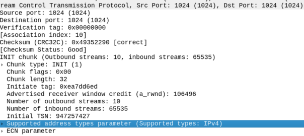
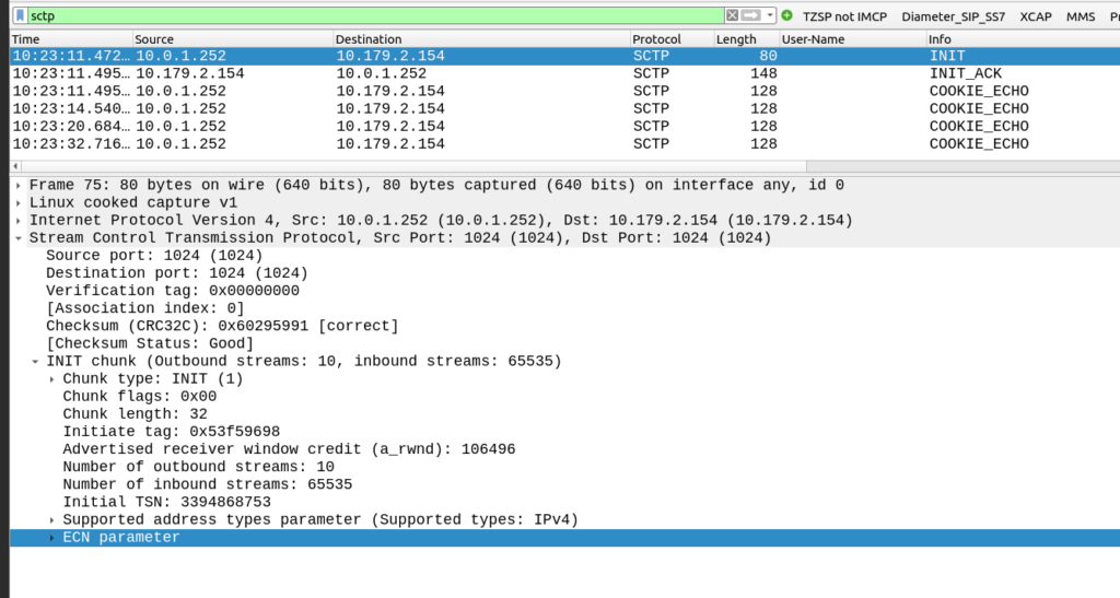
The other side of the SCTP connection didn’t like my SCTP parameters.
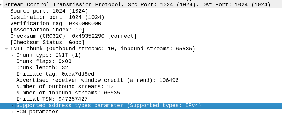
My SCTP INIT looked like this:
By default, Linux includes support for the ECN and SupportedAddressTypes parameters in the SCTP INIT.
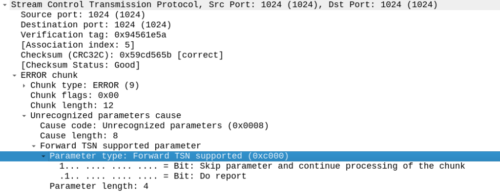
But the other side did not like this, it sent back an ERROR stating that:
Okay, apparently it doesn’t like the fact that we support Forward Transmission Sequence Numbers – So how to turn it off?
I’m using P1Sec’s PySCTP library to interact with the SCTP stack, and I couldn’t find any referneces to this in the code, but then I rememberd that PySCTP is just a wrapper for libsctp so I should be able to control it from there.
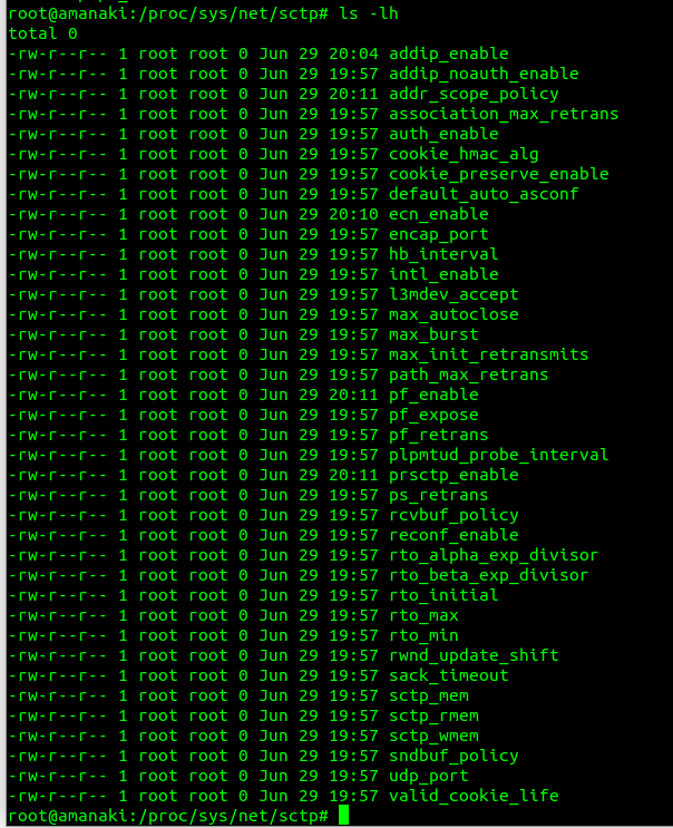
Inside /proc/sys/net/sctp we can see all the parameters we can control.
To disable the Forward TSN I need to disable the feature that controls it – Forward Transmission Sequence numbers are introduced in the Partial Reliability Extension (RFC 3758). So it was just a matter of disabling that with:
So let’s roll up our sleeves and get a Lab scenario happening,
To keep things (relatively) simple, I’ve put the eNodeB on the same subnet as the MME and Serving/Packet-Gateway.
So the traffic will flow from the eNodeB to the S/P-GW, via a simple Network Switch (I’m using a Mikrotik).
While life is complicated, I’ll try and keep this lab easy.
Experiment 1: MTU of 1500 everywhere
Network Element
MTU
Advertised MTU in PCO
1500
eNodeB
1500
Switch
1500
Core Network (S/P-GW)
1500
So everything attaches and traffic flows fine. There is no problem right?
Well, not a problem that is immediately visible.
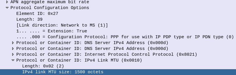
While the PCO advertises the MTU value at 1500 if we look at the maximum payload we can actually get through the network, we find that’s not the case.
This means if our end user on a mobile device tried to send a 1500 byte payload, it’d never get through.
While DNS would work, most TCP traffic would flow fine, certain UDP applications would start to fail if they were sending payloads nearing 1500 bytes.
So why is this?
Well GTP adds overhead.
8 bytes for the GTP header
8 bytes for the transport UDP header
20 bytes for the transport IPv4 header
14 bytes if our transport is using Ethernet
For a total of 50 bytes of overhead, assuming we’re not using MPLS, QinQ or anything else funky on our transport network and just using Ethernet.
So we have two options here – We can either lower the MTU advertised in our Protocol Configuration Options, or we can increase the MTU across our transport network. Let’s look at each.
Experiment 2: Lower Advertised MTU in PCO to 1300
Well this works, and looks the same as our previous example, except now we know we can’t handle payloads larger than 1300 without fragmentation.
Experiment 3: Increase MTU across transmission Network
While we need to account for the 50 bytes of overhead added by GTP, I’ve gone the safer option and upped the MTU across the transport to 1600 bytes.
With this, we can transport a full 1500 byte MTU on the UE layer, and we’ve got the extra space by enabling jumbo frames.
Obviously this requires a change on all of the transmission layer – And if you have any hops without support for this, you’ll loose packets.
Conclusions?
Well, fragmentation is bad, and we want to avoid it.
For this we up the MTU across the transmission network to support jumbo frames (greater than 1500 bytes) so we can handle the 1500 byte payloads that users want.
I generally do this with Python or via the Swagger UI for the Web UI, but here’s how we can create a fixed-line IMS subscriber in PyHSS, so we can register it with a softphone, without using EAP-AKA.
Firstly we create the AuC object for this password combo.
If you’re working with the larger SIM vendors, there’s a good chance they key material they send you won’t actually contain the raw Ki values for each card – If it fell into the wrong hands you’d be in big trouble.
Instead, what is more likely is that the SIM vendor shares the Ki generated when mixed with a transport key – So what you receive is not the plaintext version of the Ki data, but rather a ciphered version of it.
But as long as you and the SIM vendor have agreed on the ciphering to use, an the secret to protect it with beforehand, you can read the data as needed.
This is a tricky topic to broach, as transport key implementation, is not covered by the 3GPP, instead it’s a quasi-standard, that is commonly used by SIM vendors and HSS vendors alike – the A4 / K4 Transport Encryption Algorithm.
It’s made up of a few components:
K2 is our plaintext key data (Ki or OP)
K4 is the secret key used to cipher the Ki value.
K7 is the algorithm used (Usually AES128 or AES256).
It’s important when defining your electrical profile and the reuqired parameters, to make sure the operator, HSS vendor and SIM vendor are all on the same page regarding if transport keys will be used, what the cipher used will be, and the keys for each batch of SIMs.
Here’s an example from a Huawei HSS with SIMs from G&D:
We’re using AES128, and any SIMs produced by G&D for this batch will use that transport key (transport key ID 1 in the HSS), so when adding new SIMs we’ll need to specify what transport key to use.
In our last post we covered the basics of NB-IoT Non-IP Data Deliver (NIDD), and if that acronym soup wasn’t enough for you, we’re going to take a deep dive into the flows for attaching, sending, receiving and closing a NIDD session.
The attach for NIDD is very similar to the standard attach for wideband LTE, except the MME establishes a connection on the T6a Diameter interface toward the SCEF, to indicate the sub is online and available.
The NIDD Attach
The SCEF is now able to send/receive NIDD traffic from the subscriber on the T6a interface, but in reality developers don’t / won’t interact with Diameter, so the SCEF exposes the T8 API that developers can interact with to access an abstraction layer to interact with the SCEF, and then through onto the UE.
If you’re wondering what the status of Open Source SCEF implementations are, then you may have already guessed we’re working on one! PyHSS should have support for NB-IoT SCEF features in the future.
NB-IoT provides support for Non-IP Data Delivery (NIDD) over 3GPP Networks, but to handle this, some new network elements are introduced, in a home network scenario that’s the SCEF and the SCF/AS.
On the 3GPP side the SCEF it communicates to the MME via the T6a Interface, which is based upon Diameter.
On the side towards our IoT Service Consumers (in the standards referred to as “SCS/AS” or “Service Capabilities Server Application Servers” (catchy names as always), via the RESTful HTTP based T8 interface.
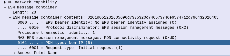
The start of the S1 Attach procedure is very similar to a regular S1 attach.
The initial S1 PDU Connectivity Request indicates in the ESM Message Container that the PDN Type is Non IP.
S1 PDU Connectivity Request from attach procedure
Other than that, the initial attach procedure looks very similar to the regular S1 attach procedure.
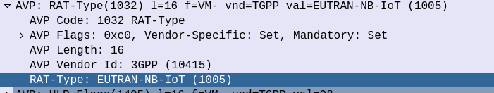
On the S6a interface the Update Location Request from the MME to the HSS indicates that this is an EUTRAN-NB-IoT Radio Access Type.
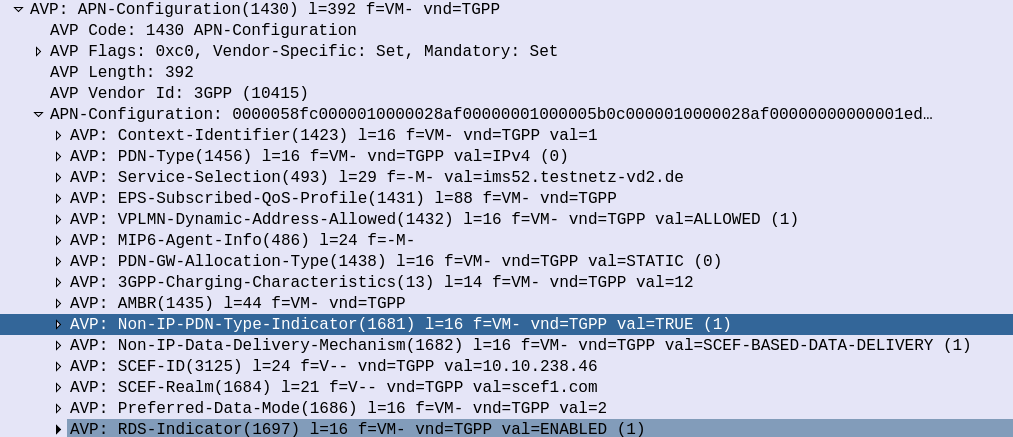
And the Update Location Answer APN Configuration contains some additional AVPs on the APN to indicate that the APN supports Non-IP-PDN-Type and that the SCEF is used for Data Delivery.
The SCEF-ID (Diameter Host) and SCEF-Realm (Diameter realm) to serve this user is also specified in the APN Configuration in the Update Location Answer.
This is how our MME determines where to send the T6a traffic.
With this, the MME sends a Connection Management Request (CMR) towards the SCEF specified in the SCEF-ID returned by the HSS.
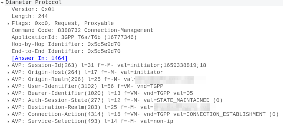
The Connection Management Request / Response
The MME now sends a Diameter T6a Connection Management Request to the SCEF in the Update Location Answer,
In it we have a Session-Id, which continues for the life of our NIDD session, the service-selection which contains our APN (In our case “non-ip”) and the User-Identifier AVP which contains the MSISDN and/or IMSI of the subscriber.
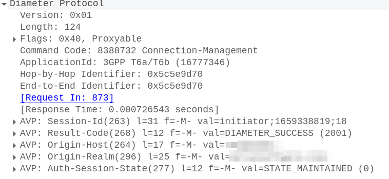
To accept this, the SCEF sends back a Connection-Management-Answer to confirm we’re all good to go:
At this point our SCEF now knows about the subscriber who’s just attached to our network, and correlates it with the APN and the session-ID.
On the S1 side the connection is confirmed and we’re ready to roll.
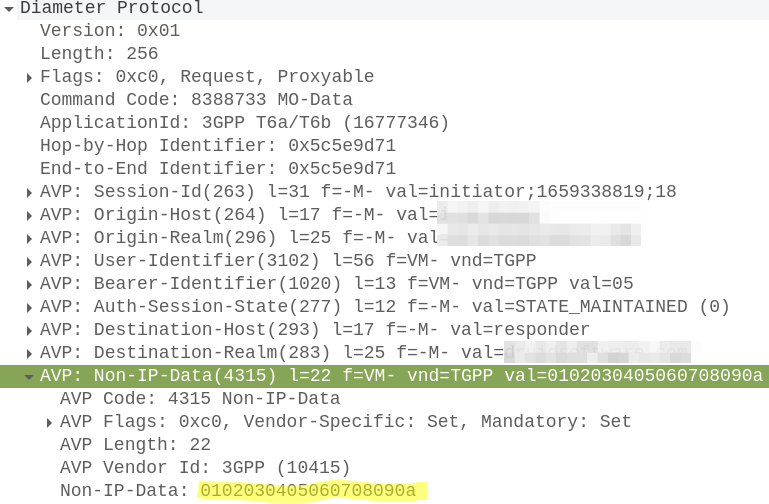
Mobile Originated Data Request / Response
When the UE wants to send NIDD it’s carried in NAS messaging, so we see an Uplink NAS transport from the UE and inside the NAS payload itself is our HEX data.
Our MME grabs this out and sends it in the form of of a Mobile-Originated-Data-Request (MODR) to the SCEF, along with the same Session-ID that was setup earlier:
At this stage our Non-IP Data is exposed over the T8 RESTful API, which we won’t cover in this post.
Note: I’m lazily posting this as its been in my drafts folder for an exceedingly long time – Before going too much further, it’s worth pointing out that eMBMS never really made it anywhere – no production networks of note use eMBMS. I started researching it and my interest petered out once I discovered I couldn’t get any UEs or hardware that supported eMBMS.
Mobile networks are designed as point to point, all traffic is unicast.
But multicast and broadcast traffic is real, and becoming more common in some applications.
In areas where users stream the same radio program, or TV show, live, each of them is consuming the same data stream, but each one gets sent a unique copy of the data, on a resource block allocated to them for reception of the data.
If we have 10 users on a cell, each streaming a 5Mbps live video, that’s 50Mbps of capacity taken up on the radio / air interface. If that stream was moved onto a eMBMS service, only 5Mbps of capacity would be used, regardless of how many people on the cell are consuming it.
For Mission Critical Push to Talk applications, the lack of broadcast/multicast support was highlighted again. For a PTT app with 10 users in a talk group, you’d need to schedule resource blocks for 10 users, and allocate 10 radio resources 10 times, send GTP packets 10 times, all to send the same data to 10 people.
So enter eMBMS – The Evolved Multimedia Broadcast and Multicast Service, providing multicast service for LTE.
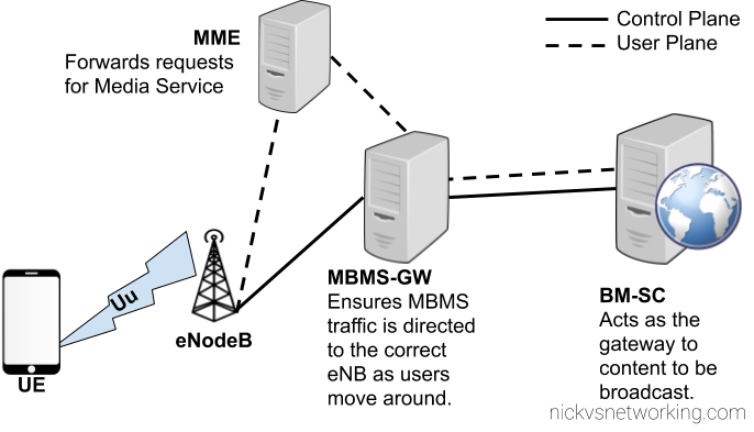
Overall Architecture
eMBMS introduces a few changes to the RAN side to handle support for a shared data channel, which is sent by the eNodeB and that UEs can listen on to get data. (More on admission control later)
From a core perspective two new network elements are introduced, the Broadcast/Multicast Service Center (BM-SC) and Multimedia Broadcast Multicast Services Gateway (MBMS GW), these elements function in much the same was the P-GW and S-GW retrospectively, but in regards to Multicast services.
Like so many 3GPP specs before it, MBMS relies on GTP for transporting the data to be distributed, and relies on GTPv2-C for control plane data.
BM-SC – Broadcast Media Service Centre
The Broadcast Multicast Service Centre acts as the gateway between content providers (providing streams of data to be distributed) and the EPC.
The BM-SC sets up eMBMS sessions and pulls broadcast data from the content providers and collects receipts from subscribers of some streams to charge / track consumption of the services.
In this regard the BM-SC is akin to the P-GW, which as the border for the EPC and external networks, except it’s largely unidirectional.
MBMS Gateway
The MBMS Gateway (MBMS-GW) encapsulates the broadcast data stream from the BM-SC and encapsulates it into GTP packets to be distributed to eNBs across the network.
The MBMS-GW allocates a multicast transport address for each broadcast data stream?
MME Interaction
For this a new interface is introduced on the MME – the Sm interface, which interconnects the MME and the MBMS-Gateways assigned to it.
I started seeing this error the other day when running CDRsv1.GetCDRs on the CGrateS API:
SERVER_ERROR: unexpected end of JSON input
It seemed related to certain CDRs in the cdrs table of StoreDB.
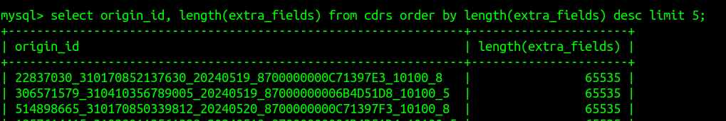
After some digging, I found the stupid simple problem:
I’d written too much data to extra_fields, leading MySQL to cut off the data mid way through, meaning it couldn’t be reconstructed as JSON by CGrateS again.
Like the rounding issue I had, this wasn’t an issue with CGrateS but with MySQL.
Quick fix:
sudo mysql cgrates -e "ALTER TABLE cdrs MODIFY extra_fields LONGTEXT;"
And new fields can exceed this length without being cut off.