For a long time I’ve run my own backups to a portable hard drive using Duplicity / Dejavu.
It’s worked really well, it’s dammed slow to pull back a file I’ve accidentally deleted, or need an old version of (which I probably go back to every 6 months or so), but it’s fast to backup, and I do that a whole lot more than I recover. I’ve even used it when swapping laptops to move all my data as a test, plus the slowness of recovery acts as a good deterrent to me doing dumb things like dropping partition tables and needing to use the backup.
That worked fine as an individual but at work the team is generating more and more data, and I needed a way to backup all our shared drives and docs, which is constantly growing, which means I needed a solution that didn’t involve just buying a lot of drives at crack money.
So I got a tape deck.
It seemed like a good solution; I like that I can eject the tape, and that I can just append to tape with (minimal) risk of nuking the data already there. These two points were how I justified it logically, but it’s also weird tech I haven’t used before (which was the main driver for me wanting to use it).
My first few problems with tape are:
- I have more data than a single tape can handle
- I have more data than I have free storage capacity to buffer it
- I have no idea how to use a tape drive or how to connect it
The Bits
LTO-6 seems like a sweet spot for tape storage at 2.5TB uncompressed (Sure you can buy LTO-10 drives, with 40TB capacity, but they cost more than my car), however because this is an experiment I picked up an LTO-4 (800GB uncompressed) tape drive for $50, plus 10 tapes ($60 / $6 each) so I could try it all out.
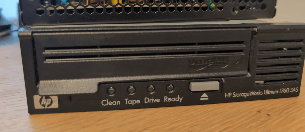
The tape drive has SAS connectors on it, my homelab server has SAS drives in it (A Dell R630 that lives under the couch in my office my dog sleep on when I’m at work), but there’s no way I’m fitting this chonky tape drive into a 2.5″ disk bay.
Searching online told me to buy a “Dell 0T93GD T93GD LSI 9300-8e 12Gbps Dual-Port External SAS HBA Controller” which I duly spent $55 on without really understanding what exactly an HBA is.
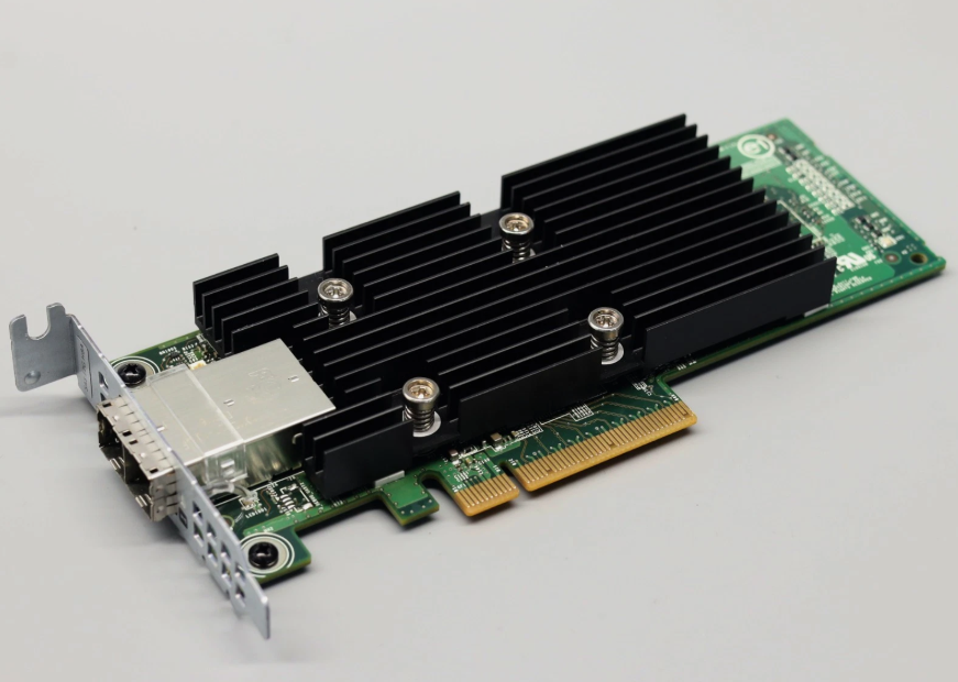
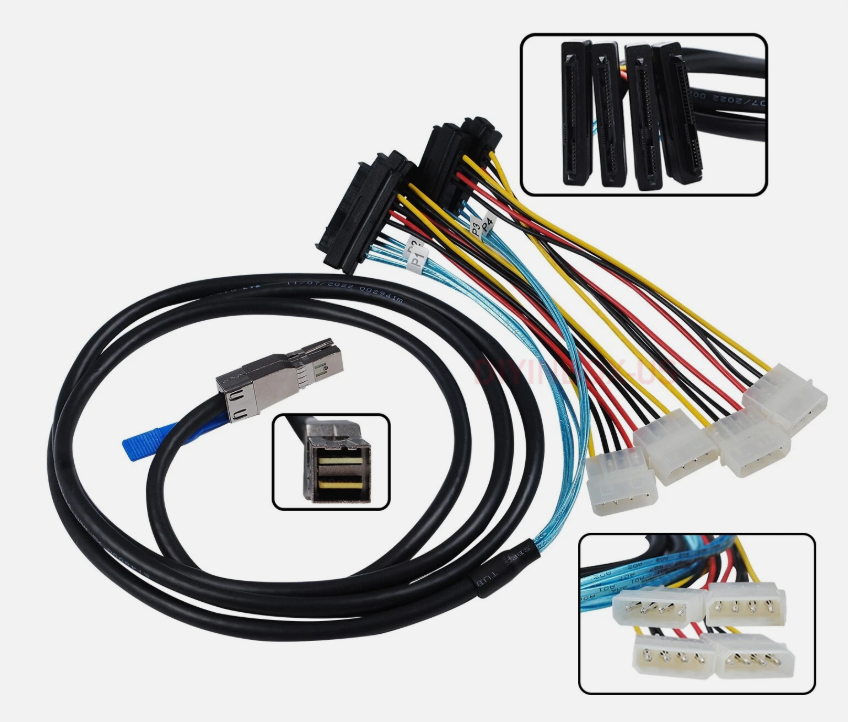
Being an HBA it’s got the Mini-SAS HD (SFF-8644) connector, which does not look like the SAS connector on my tape drive, so I needed a Mini-SAS HD (SFF-8644) to 29Pin SAS cable, and I grabbed a long one as the tape drive lives on the desk not under the couch.
Wiring it Up
I used my advanced plugging skills to plug things in. I’m not really sure why I added a heading here, I just plugged the female SAS cable into the tape drive, hooked an ATX power supply with a paperclip shoved in it into the ATX supply to turn it on, and plugged the other end into the server.
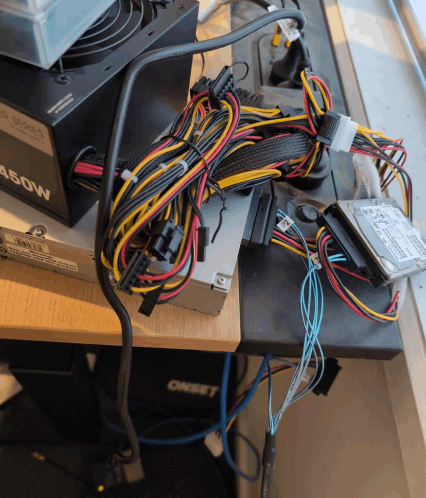
In the end I grabbed a spare 10K SAS magnetic drive with 1.8T on it, and used that as a cache on the same HBA, so I’d pull the files onto there, an then push them sequentially to the tape.
Then inside Proxmox I passed the PCI device for the HBA adapter into the VM.
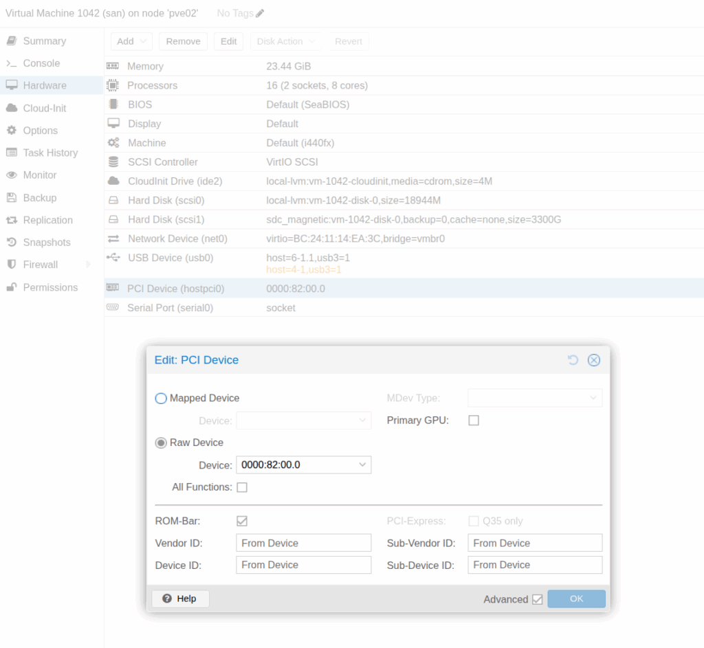
Linux just detected it as a tape drive, and we’re good to go.
The next issue I ran into was read and write speeds of the magnetic cache drive, and the tape.
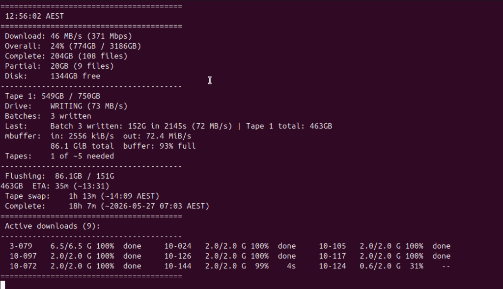
The fastest I could pull from Google and write to disk was ~480Mbps (Okay because we’re dealing with storage for the most part, I’ll deal in MB/s which is ~58MB/s), I’ve got more capacity on the link to Google, but not on the drive which tops out around here.
The tape writes at a pretty sustained 72MB/s, so tape writes faster than the disk it’s reading from, which meant the tape jobs finished ~20% faster than the cache filled, this is good because it allowed me to sleep without needing to swap tapes in the middle of the night or fill the cache disk.
I tried Baccula but it’s not great for this “I have a bunch of data to dump onto a drive” problem, so I instead used tar which stands for “Tape Archive” (who knew) to compress the files and put them all onto tapes.
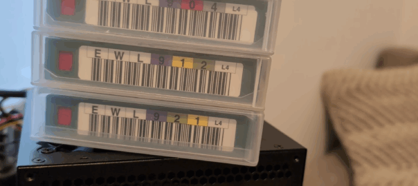
The write took a good long while – ~20 hours, but I validated each one as I went and created a file manifest so if I need a particular archive I know which tape it’s on (labeled with advanced Sharpie).
So the result of the experiment?
Well, the data is backed up, and I now have a good long term storage solution, I also backed up all the family photo albums,
Will I buy an LTO-6 or LTO-7 drive and use this more frequently? Maybe. But did I enjoy learning about it and messing around with a weird storage format, you betcha.