Give me a lever long enough and a fulcrum on which to place it, and I shall move the world.
For me, the equivalent would be:
Give me a packet capture of the problem occurring and a standards document against which to compare it, and I shall debug the networking world.
And if you’re like me, there’s a good chance when things are really not going your way, you roll up your sleeves, break out Wireshark and the standards docs and begin the painstaking process of trying to work out what’s not right.
Today’s problem involved a side by side comparison between a pcap of a known good call, and one which is failing, so I just had to compare the two, which is slow and fairly error-prone,
So I started looking for something to diff PCAPs easily. The data I was working with was ASN.1 encoded so I couldn’t export as text like you can with HTTP or SIP based protocols and compare it that way.
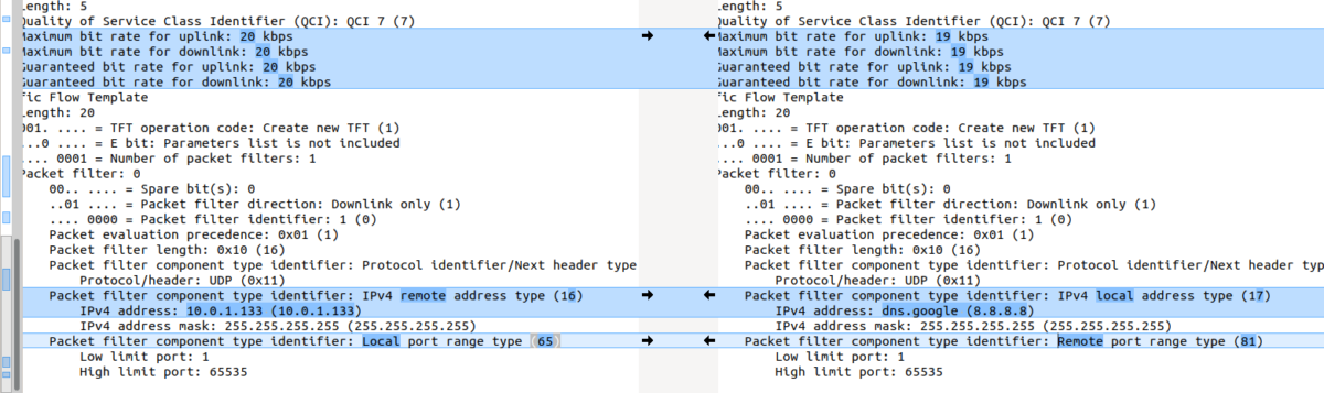
In the end I stumbled across something even better to compare frames from packet captures side by side, with the decoding intact!
Turns out yo ucan copy the values including decoding from within Wireshark, which means you can then just paste the contents into a diff tool (I’m using the fabulous Meld on Linux, but any diff tool will do including diff itself) and off you go, side-by-side comparison.
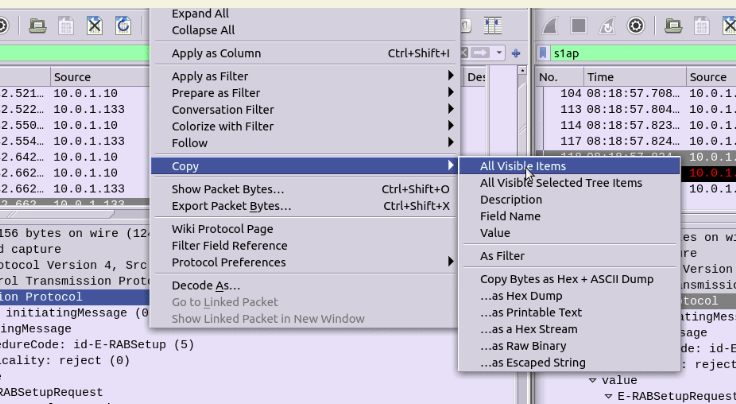
Select the first packet/frame you’re interested in (or even just the section), expand the subkeys, right click, copy “All Visible items”. This copy contains all the decoded data, not just the raw bytes, which is what makes it so great.
Next paste it into your diff tool of choice, repeat with the one to compare against, scroll past the data you know is going to be different (session IDs, IPs, etc) and ta-da, there’s the differences.
One feature I’m pretty excited to share is the addition of a single config file for defining how PyHSS functions,
In the past you’d set variables in the code or comment out sections to change behaviour, which, let’s face it – isn’t great.
Instead the config.yaml file defines the PLMN, transport time (TCP or SCTP), the origin host and realm.
We can also set the logging parameters, SNMP info and the database backend to be used,
HSS Parameters
 hss:
   transport: "SCTP"
   #IP Addresses to bind on (List) - For TCP only the first IP is used, for SCTP all used for Transport (Multihomed).
   bind_ip: ["10.0.1.252"]
 #Port to listen on (Same for TCP & SCTP)
   bind_port: 3868
 #Value to populate as the OriginHost in Diameter responses
   OriginHost: "hss.localdomain"
 #Value to populate as the OriginRealm in Diameter responses
   OriginRealm: "localdomain"
 #Value to populate as the Product name in Diameter responses
   ProductName: "pyHSS"
 #Your Home Mobile Country Code (Used for PLMN calcluation)
   MCC: "999"
   #Your Home Mobile Network Code (Used for PLMN calcluation)
   MNC: "99"
 #Enable GMLC / SLh Interface
   SLh_enabled: True


 logging:
   level: DEBUG
   logfiles:
     hss_logging_file: log/hss.log
     diameter_logging_file: log/diameter.log
     database_logging_file: log/db.log
   log_to_terminal: true

 database:
   mongodb:
     mongodb_server: 127.0.0.1
     mongodb_username: root
     mongodb_password: password
     mongodb_port: 27017

 Stats Parameters
 redis:
   enabled: True
   clear_stats_on_boot: False
   host: localhost
   port: 6379
 snmp:
   port: 1161
   listen_address: 127.0.0.1
I’d tried in the past to use the USB port on the Mikrotik, an external HDD and the SMB server in RouterOS, to act as a simple NAS for sharing files on the home network. And the performance was terrible.
This is because the device is a Router. Not a NAS (duh). And everything I later read online confirmed that yes, this is a router, not a NAS so stop trying.
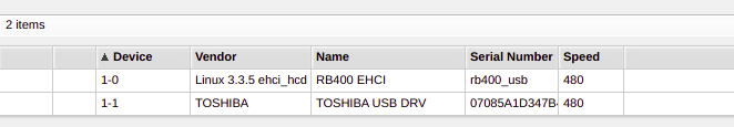
But I recently got a new Mikrotik CRS109, so now I have a new Mikrotik, how bad is the SMB file share performance?
To test this I’ve got a USB drive with some files on it, an old Mikrotik RB915G and the new Mikrotik CRS109-8G-1S-2HnD-IN, and compared the time it takes to download a file between the two.
Mikrotik Routerboard RB951G
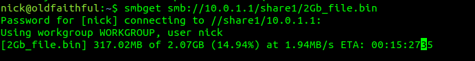
While pulling a 2Gb file of random data from a FAT formatted flash drive, I achieved a consistent 1.9MB/s (15.2 Mb/s)
nick@oldfaithful:~$ smbget smb://10.0.1.1/share1/2Gb_file.bin
 Password for [nick] connecting to //share1/10.0.1.1:
 Using workgroup WORKGROUP, user nick
 smb://10.0.1.1/share1/2Gb_file.bin
 Downloaded 2.07GB in 1123 seconds
Mikrotik CRS109
In terms of transfer speed, a consistent 2.8MB/s (22.4 Mb/s)
nick@oldfaithful:~$ smbget smb://10.0.1.1/share1/2Gb_file.bin
 Password for [nick] connecting to //share1/10.0.1.1:
 Using workgroup WORKGROUP, user nick
 smb://10.0.1.1/share1/2Gb_file.bin
 Downloaded 2.07GB in 736 seconds
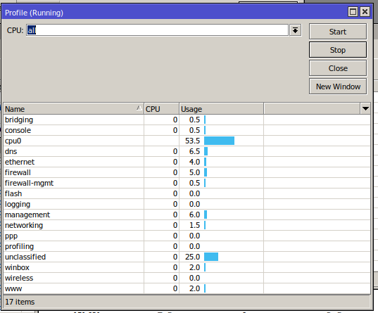
Profiler shows 25% CPU usage on “other”, which drops down as soon as the file transfers stop,
So better, but still not a NAS (duh).
The Verdict
Still not a NAS. So stop trying to use it as a NAS.
As my download speed is faster than 22Mbps I’d just be better to use cloud storage.
I’ve been adding SNMP support to an open source project I’ve been working on (PyHSS) to generate metrics / performance statistics from it, and this meant staring down SNMP again, but this time I’ve come up with a novel way to handle SNMP, that made it much less painful that normal.
The requirement was simple enough, I already had a piece of software I’d written in Python, but I had a need to add an SNMP server to get information about that bit of software.
For a little more detail – PyHSS handles Device Watchdog Requests already, but I needed a count of how many it had handled, made accessible via SNMP. So inside the logic that does this I just increment a counter in Redis;
In the code example above I just add 1 (increment) the Redis key ‘Answer_280_attempt_count’.
The beauty is that that this required minimal changes to the rest of my code – I just sprinkled in these statements to increment Redis keys throughout my code.
Now when that existing function is run, the Redis key “Answer_280_attempt_count” is incremented.
So I ran my software and the function I just added the increment to was called a few times, so I jumped into redis-cli to check on the values;
And just like that we’ve done all the heavy lifting to add SNMP to our software.
For anything else we want counters on, add the increment to your code to store a counter in Redis with that information.
So next up we need to expose our Redis keys via SNMP,
Then when you run it, presto, you’re exposing that data via SNMP.
You can verify it through SNMP walk or start integrating it into your NMS, in the above example OID 1.3.6.1.2.1.1.1.0.2, contains the value of Answer_280_attempt_count from Redis, and with that, you’re exposing info via SNMP, all while not really having to think about SNMP.
*Ok, you still have to sort which OIDs you assign for what, but you get the idea.
It’s 2021, and everyone loves Containers; Docker & Kubernetes are changing how software is developed, deployed and scaled.
And yet so much of the Telco world still uses bare metal servers and dedicated hardware for processing.
So why not use Containers or VMs more for VoIP applications?
Disclaimer – When I’m talking VoIP about VoIP I mean the actual Voice over IP, that’s the Media Stream, RTP, the Audio, etc, not the Signaling (SIP). SIP is fine with Containers, it’s the media that has a bad time and that this post focuses on,
Virtualization Fundamentals
Once upon a time in Development land every application ran on it’s own server running in a DC / Central Office.
This was expensive to deploy (buying servers), operate (lots of power used) and maintain (lots of hardware to keep online).
Each server was actually sitting idle for a large part of the time, with the application running on it only using a some of the available resources some of the time.
One day Virtualization came and suddenly 10 physical servers could be virtualized into 10 VMs.
These VMs still need to run on servers but as each VM isn’t using 100% of it’s allocated resources all the time, instead of needing 10 servers to run it on you could run it on say 3 servers, and even do clever things like migrate VMs between servers if one were to fail.
VMs share the resources of the server it’s running on.
A server running VMs (Hypervisor) is able to run multiple VMs by splitting the resources between VMs.
If a VM A wants to run an operation at the same time a VM B & VM C, the operations can’t be run on each VM at the same time* so the hypervisor will queue up the requests and schedule them in, typically based on first-in-first out or based on a resource priority policy on the Hypervisor.
This is fine for a if VM A, B & C were all Web Servers. A request coming into each of them at the same time would see the VM the Hypervisor schedules the resources to respond to the request slightly faster, with the other VMs responding to the request when the hypervisor has scheduled the resources to the respective VM.
VoIP is an only child
VoIP has grown up on dedicated hardware. It’s an only child that does not know how to share, because it’s never had to.
Having to wait for resources to be scheduled by the Hypervisor to to VM in order for it to execute an operation is fine and almost unnoticeable for web servers, it can have some pretty big impacts on call quality.
If we’re running RTPproxy or RTPengine in order to relay media, scheduling delays can mean that the media stream ends up “bursty”.
RTP packets needing relaying are queued in the buffer on the VM and only relayed when the hypervisor is able to schedule resources, this means there can be a lot of packet-delay-variation (PDV) and increased latency for services running on VMs.
VMs and Containers both have this same fate, DPDK and SR-IOV assist in throughput, but they don’t stop interrupt headaches.
VMs that deprive other VMs on the same host of resources are known as “Noisy neighbors”.
The simple fix for all these problems? There isn’t one.
Each of these issues can be overcome, dedicating resources, to a specific VM or container, cleverly distributing load, but it is costly in terms of resources and time to tweak and implement, and some of these options undermine the value of virtualization or containerization.
As technology marches forward we have scenarios where Kubernetes can expose FPGA resources to pass them through to Pods, but right now, if you need to transcode more than ~100 calls efficiently, you’re going to need a hardware device.
And while it can be done by throwing more x86 / ARM compute resources at the problem, hardware still wins out as cheaper in most instances.
Australia is a strange country; As a kid I was scared of dogs, and in response, our family got a dog.
This year started off with adventures working with ASN.1 encoded data, and after a week of banging my head against the table, I was scared of ASN.1 encoding.
But now I love dogs, and slowly, I’m learning to embrace ASN.1 encoding.
What is ASN.1?
ASN.1 is an encoding scheme.
The best analogy I can give is to image a sheet of paper with a form on it, the form has fields for all the different bits of data it needs,
Each of the fields on the form has a data type, and the box is sized to restrict input, and some fields are mandatory.
Now imagine you take this form and cut a hole where each of the text boxes would be.
We’ve made a key that can be laid on top of a blank sheet of paper, then we can fill the details through the key onto the blank paper and reuse the key over and over again to fill the data out many times.
When we remove the key off the top of our paper, and what we have left on the paper below is the data from the form. Without the key on top this data doesn’t make much sense, but we can always add the key back and presto it’s back to making sense.
While this may seem kind of pointless let’s look at the advantages of this method;
The data is validated by the key – People can’t put a name wherever, and country code anywhere, it’s got to be structured as per our requirements. And if we tried to enter a birthday through the key form onto the paper below, we couldn’t.
The data is as small as can be – Without all the metadata on the key above, such as the name of the field, the paper below contains only the pertinent information, and if a field is left blank it doesn’t take up any space at all on the paper.
It’s these two things, rigidly defined data structures (no room for errors or misinterpretation) and the minimal size on the wire (saves bandwidth), that led to 3GPP selecting ASN.1 encoding for many of it’s protocols, such as S1, NAS, SBc, X2, etc.
It’s also these two things that make ASN.1 kind of a jerk; If the data structure you’re feeding into your ASN.1 compiler does not match it will flat-out refuse to compile, and there’s no way to make sense of the data in its raw form.
But working with a super simple ASN.1 definition you’ve created is one thing, using the 3GPP defined ASN.1 definitions is another,
With the aid of the fantastic PyCrate library, which is where the real magic happens, and this was the nut I cracked this week, compiling a 3GPP ASN.1 definition and communicating a standards-based protocol with it.
So dedicated appliances are dead and all our network functions are VMs or Containers, but there’s a performance hit when going virtual as the L2 processing has to be handled by the Hypervisor before being passed onto the relevant VM / Container.
If we have a 10Gb NIC in our server, we want to achieve a 10Gbps “Line Speed” on the Network Element / VNF we’re running on.
When we talked about appliances if you purchased an P-GW with 10Gbps NIC, it was a given you could get 10Gbps through it (without DPI, etc), but when we talk about virtualized network functions / network elements there’s a very real chance you won’t achieve the “line speed” of your interfaces without some help.
When you’ve got a Network Element like a S-GW, P-GW or UPF, you want to forward packets as quickly as possible – bottlenecks here would impact the user’s achievable speeds on the network.
To speed things up there are two technologies, that if supported by your software stack and hardware, allows you to significantly increase throughput on network interfaces, DPDK & SR-IOV.
DPDK – Data Plane Development Kit
Usually *Nix OSs handle packet processing on the Kernel level. As I type this the packets being sent to this WordPress server by Firefox are being handled by the Linux 5.8.0-36-generic kernel running on my machine.
The problem is the kernel has other things to do (interrupts), meaning increased delay in processing (due to waiting for processing capability) and decreased capacity.
DPDK shunts this processing to the “user space” meaning your application (the actual magic of the VNF / Network Element) controls it.
To go back to me writing this – If Firefox and my laptop supported DPDK, then the packets wouldn’t traverse the Linux kernel at all, and Firefox would be talking directly to my NIC. (Obviously this isn’t the case…)
So DPDK increases network performance by shifting the processing of packets to the application, bypassing the kernel altogether. You are still limited by the CPU and Memory available, but with enough of each you should reach very near to line speed.
SR-IOV – Single Root Input Output Virtualization
Going back to the me writing this analogy I’m running Linux on my laptop, but let’s imagine I’m running a VM running Firefox under Linux to write this.
If that’s the case then we have an even more convolted packet processing chain!
I type the post into Firefox which sends the packets to the Linux kernel, which waits to be scheduled resources by the hypervisor, which then process the packets in the hypervisor kernel before finally making it onto the NIC.
We could add DPDK which skips some of these steps, but we’d still have the bottleneck of the hypervisor.
With PCIe passthrough we could pass the NIC directly to the VM running the Firefox browser window I’m typing this, but then we have a problem, no other VMs can access these resources.
SR-IOV provides an interface to passthrough PCIe to VMs by slicing the PCIe interface up and then passing it through.
My VM would be able to access the PCIe side of the NIC, but so would other VMs.
So that’s the short of it, SR-IOR and DPDK enable better packet forwarding speeds on VNFs.
So a problem had arisen, carriers wanted to change certain carrier related settings on devices (Specifically the Carrier Config Manager) in the Android ecosystem. The Android maintainers didn’t want to open the permissions to change these settings to everyone, only the carrier providing service to that device.
And if you purchased a phone from Carrier A, and moved to Carrier B, how do you manage the permissions for Carrier B’s app and then restrict Carrier A’s app?
The carrier loads a certificate onto the SIM Cards, and signing Android Apps with this certificate, allowing the Android OS to verify the certificate on the card and the App are known to each other, and thus the carrier issuing the SIM card also issued the app, and presto, the permissions are granted to the app.
Carriers have full control of the UICC, so this mechanism provides a secure and flexible way to manage apps from the mobile network operator (MNO) hosted on generic app distribution channels (such as Google Play) while retaining special privileges on devices and without the need to sign apps with the per-device platform certificate or preinstall as a system app.
I’ve written a playbook that provisions some server infrastructure, however one of the steps is to change the hostname.
A common headache when changing the hostname on a Linux machine is that if the hostname you set for the machine, isn’t in the machine’s /etc/hosts file, then when you run sudo su or su, it takes a really long time before it shows you the prompt as the machine struggles to do a DNS lookup for it’s own hostname and fails,
This becomes an even bigger problem when you’re using Ansible to setup these machines, Ansible times out when changing the hostname;
Simple fix, edit the /etc/ansible/ansible.cfg file and include
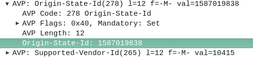
The Origin-State-Id AVP solves a kind of tricky problem – how do you know if a Diameter peer has restarted?
It seems like a simple problem until you think about it. One possible solution would be to add an AVP for “Recently Rebooted”, to be added on the first command queried of it from an endpoint, but what if there are multiple devices connecting to a Diameter endpoint?
The Origin-State AVP is a strikingly simple way to solve this problem. It’s a constantly incrementing counter that resets if the Diameter peer restarts.
If a client receives a Answer/Response where the Origin-State AVP is set to 10, and then the next request it’s set to 11, then the one after that is set to 12, 13, 14, etc, and then a request has the Origin-State AVP set to 5, the client can tell when it’s restarted by the fact 5 is lower than 14, the one before it.
It’s a constantly incrementing counter, that allows Diameter peers to detect if the endpoint has restarted.
Simple but effective.
You can find more about this in RFC3588 – the Diameter Base Protocol.
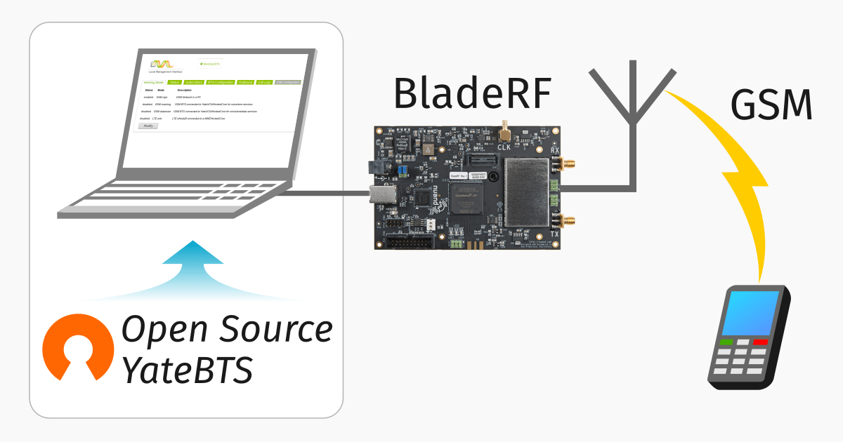
I did a post yesterday on setting up YateBTS, I thought I’d cover the basic setup I had to do to get everything humming;
Subscribers
In order to actually accept subscribers on the network you’ll need to set a Regex pattern to match the prefix of the IMSI of the subscribers you want to connect to the network,
In my case I’m using programmable SIMs with MCC / MNC 00101 so I’ve put the regex pattern matching starting with 00101.
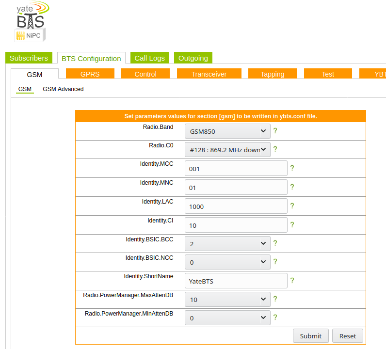
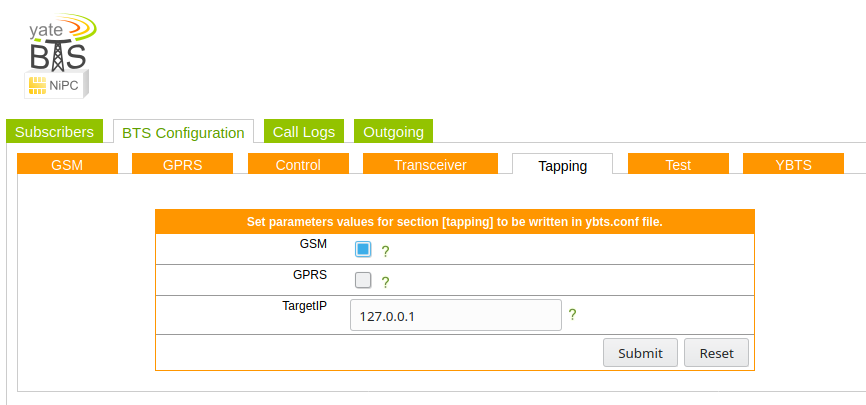
BTS Configuration
Next up you need to set the operating frequency (radio band), MNC and MCC of the network. I’m using GSM850,
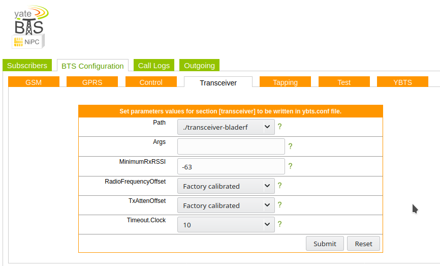
Next up we’ll need to set the device we’re going to use for the TX/RX, I’m using a BladeRF Software Defined Radio, so I’ve selected that from the path.
Optional Steps
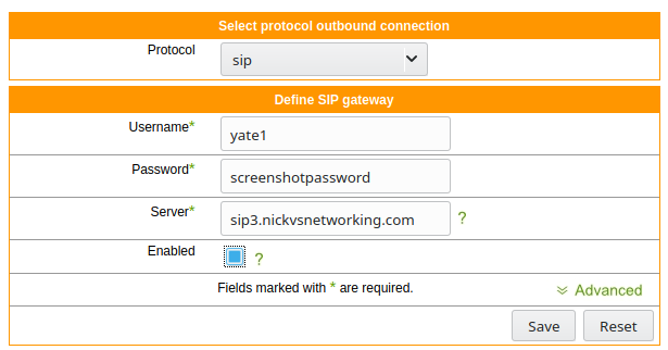
I’ve connected Yate to a SIP trunk so I can make and receive calls,
I’ve also put a tap on the GSM signaling, so I can see what’s going on, to access it just spin up Wireshark and filter for GSMMAP
A lot of the Yate tutorials are a few years old, so I thought I’d put together the steps I used on Ubuntu 18.04:
Installing Yate
apt-get install subversion autoconf build-essential
cd /usr/src svn checkout http://voip.null.ro/svn/yate/trunk yate
cd yate
./autogen.sh
./configure
make
make install-noapi
I wrote about using Ansible to automate Kamailio config management, Ansible is great at managing VMs or bare metal deployments, but for Containers using Docker to build and manage the deployments is where it’s at.
I’m going to assume you’ve got Docker in place, if not there’s heaps of info online about getting started with Docker.
The Dockerfile
The Kamailio team publish a Docker image for use, there’s no master branch at the moment, so you’ve got to specify the version; in this case kamailio:5.3.3-stretch.
Once we’ve got that we can start on the Dockerfile,
For this example I’m going to include
#Kamailio Test Stuff
FROM kamailio/kamailio:5.3.3-stretch

#Copy the config file onto the Filesystem of the Docker instance
COPY kamailio.cfg /etc/kamailio/

#Print out the current IP Address info
RUN ip add

#Expose port 5060 (SIP) for TCP and UDP
EXPOSE 5060
EXPOSE 5060/udp
Once the dockerfile is created we can build an image,
docker image build -t kamtest:0.1 .
And then run it,
docker run kamtest:0.1
Boom, now Kamailio is running, with the config file I pushed to it from my Dockerfile directory,
Now I can setup a Softphone on my local machine and point it to the IP of the Docker instance and away we go,
Where the real power here comes in is that I can run that docker run command another 10 times, and have another 10 Kamailio instannces running.
Tie this in with Kubernetes or a similar platform and you’ve got a way to scale and manage upgrades unlike anything you’d get on Bare Metal or VMs.
I had a few headaches getting the example P-CSCF example configs from the Kamailio team to run, recent improvements with the IPsec support and code evolution meant that the example config just didn’t run.
So, after finally working out the changes I needed to make to get Kamailio to function as a P-CSCF, I took the plunge and made my first pull request on the Kamailio project.
This series of post covers RF Planning using Forsk Atoll. We cover the basics of RF Planning in the process of learning how to use the software.
Forsk Atoll is software for RF Planning and Optimization of mobile networks.
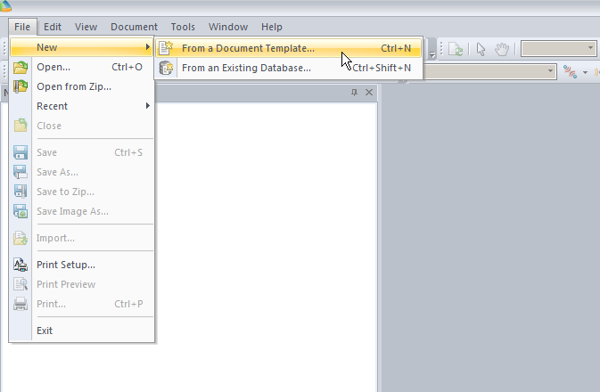
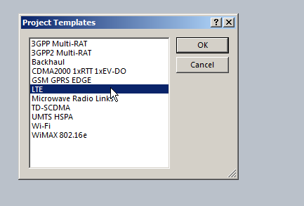
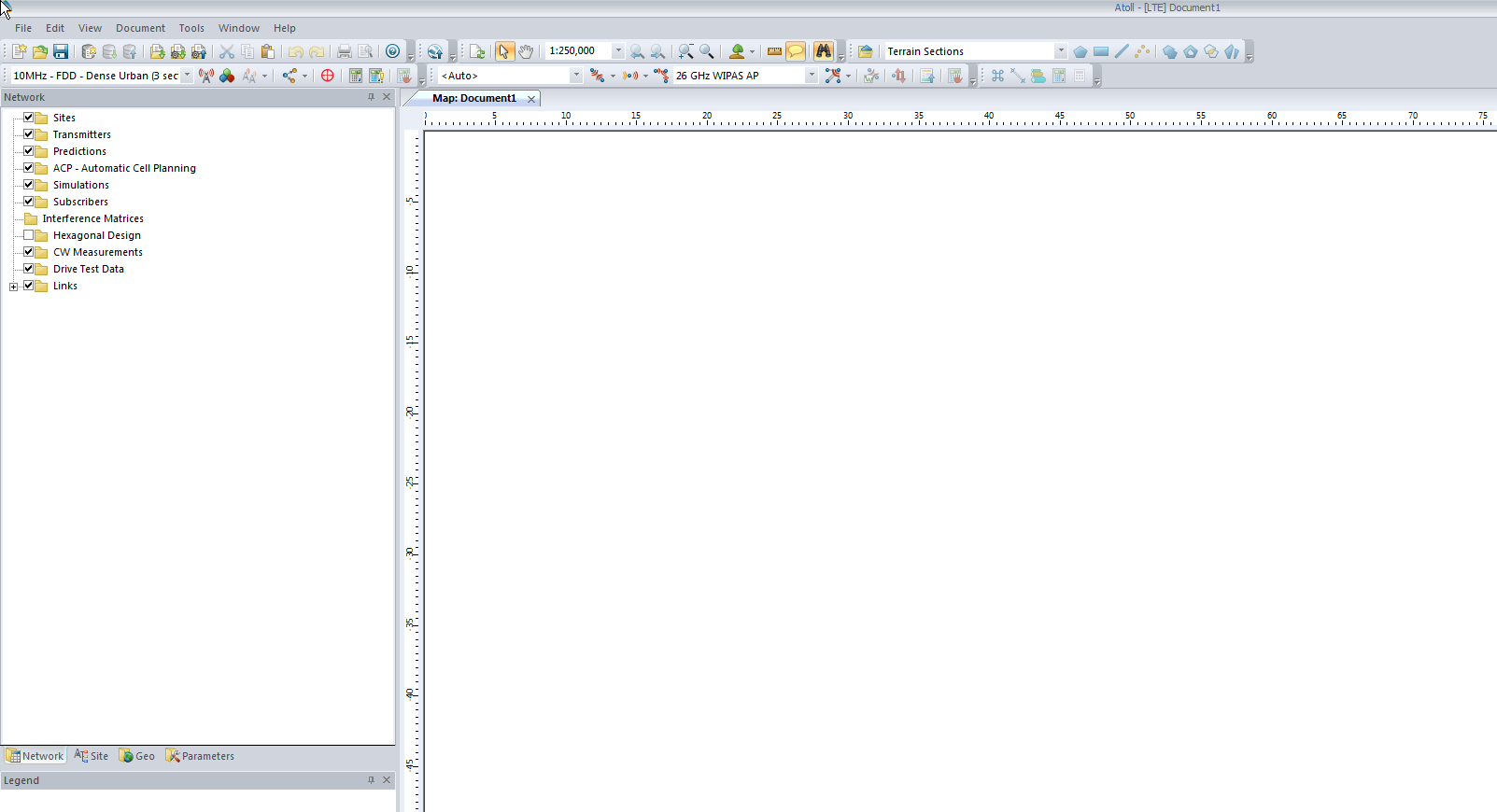
We’ll start by creating a new document from template:
In our example we’re working with LTE, so, we’ll pick the LTE template.
(The templates setup the basic information on what we’re looking at, prediction models and defaults.)
So now we’ll be looking at a blank white document, showing our map, with no data on it, Atoll doesn’t know if the area is hilly, heavily populated, densely treed, what we’re dealing with is a flat void with no features – “flatland” a perfect place to start.
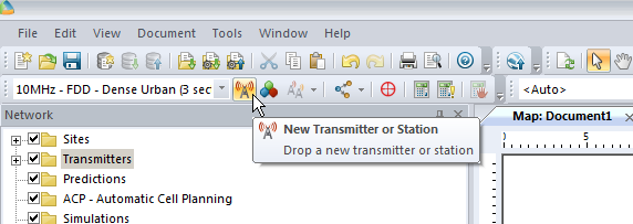
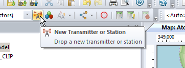
We’ll add an eNodeB (Transmitter Station and Site) from the top menu bar, clicking the transmitter icon to add a new Transmitter or Station.
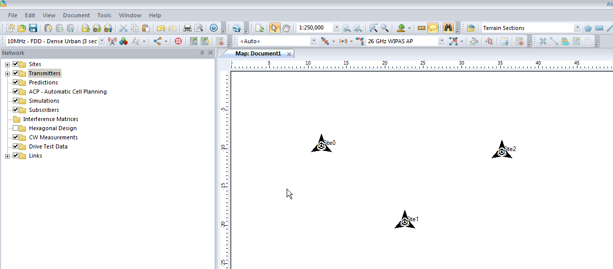
Now we’ll click in the white of our map to place the transmitter site, and repeat this a few times.
Now we’ve added a few transmitter sites, let’s take a bit of a look at one.
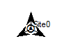
If we take a closer look we’ll see it’s actually created us a 3 sector site, and each of the arrows coming from the site is a cell sector.
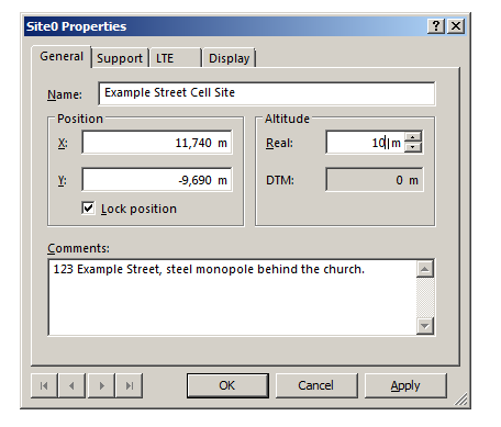
Double clicking on the transmitter will allow us to change the basic info about the site, such as it’s location, as well as display parameters, etc.
In the General tab I’ve renamed Site0 to “Example Street Cell Site”, given it an altitude (for the base of the site) and some comments,
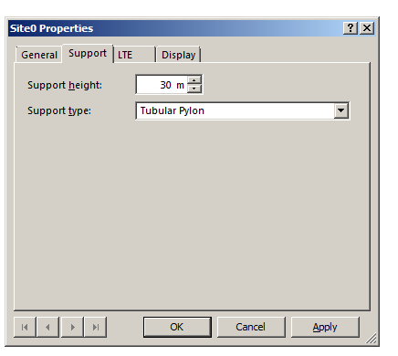
In the Support tab I’ve put some information about the support structure the antennas are one, in our case it’s on a 30m pylon / monopole.
In the LTE tab we can specify S1 throughput (backhaul) and in the Display tab we can set the color / icon used to display this site, but we’ll keep it simple for now and confirm these changes by pressing OK.
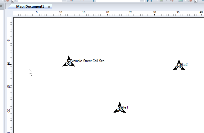
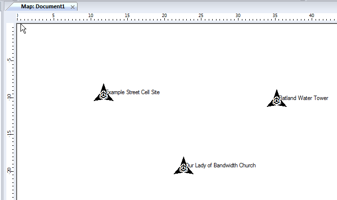
We can give each of our other Transmitters a bit of basic info, again, same process, double click on them and add some info:
So in my example I’ve got 3 transmitter sites, labeled and each given a bit of basic info. The main thing we need to have correct for each site is the location (In our case we’re placing them anywhere so it doesn’t matter), the height of the site (Altitude -Real) and the height of the structure (Support Height) the antennas are on.
Now we’ve got our 3 cell sites in our imaginary town devoid of any features, let’s get some coverage predictions for the inhabitants of desolate featureless town!
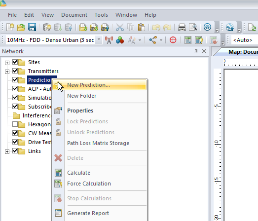
We’ll right click on Predictions and select “New Prediction”,
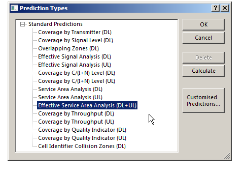
There’s a lot of different prediction types, but let’s look at the Effective Service Area Analysis for Uplink and Downlink from our eNodeBs.
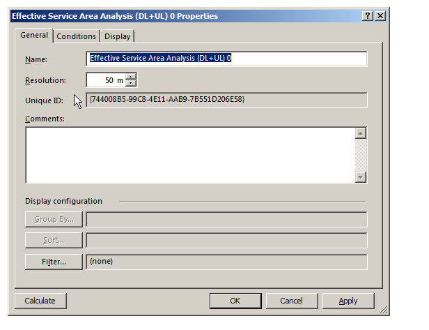
We’ll be asked to give this coverage prediction a name, and also specify a Resolution – The higher the resolution the more processing time but the higher the accuracy calculated.
At 50m it means Atoll will split the map into 50m squares and calculate the coverage in each square. This would be suitable for planning in really rural areas where you want a rough idea of footprint, but for In Building Coverage you’d want far more resolution, so you might want select 5m resolution say.
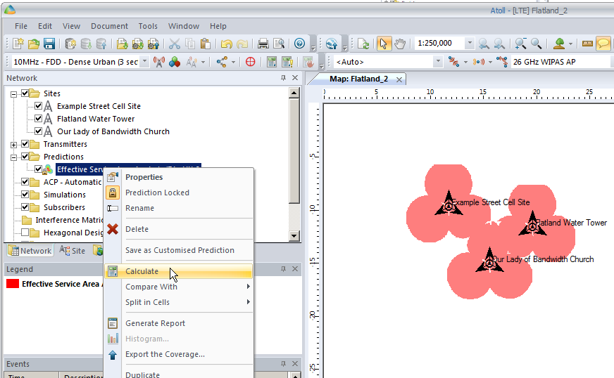
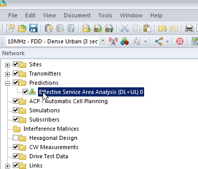
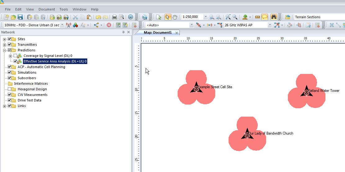
We’ll click Ok and now if we expand “Predictions” we’ll see our catchily named “Effective Service Area Analysis” there.
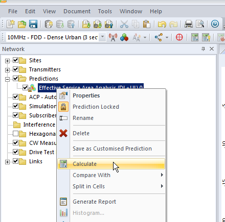
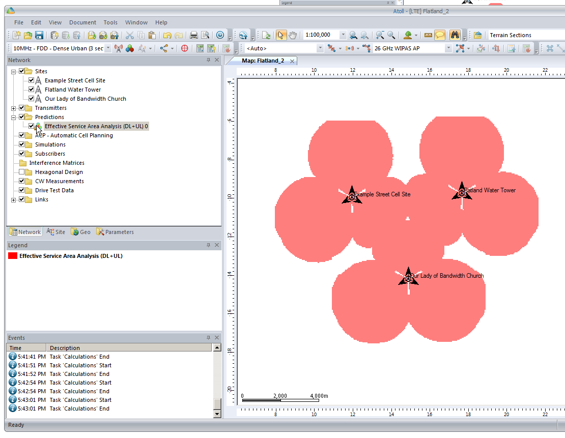
By right clicking on our prediction we can select “Calculate” and presto, we’ll have a prediction of service area from each of our cells,
Each of those pink cherry blobs represents the effective usable area of coverage provided by our network.
We may have some unhappy customers looking at this, our users will only be able to use their devices around Fake Street, Flatland Water Tower and the Our Lady of Bandwidth church.
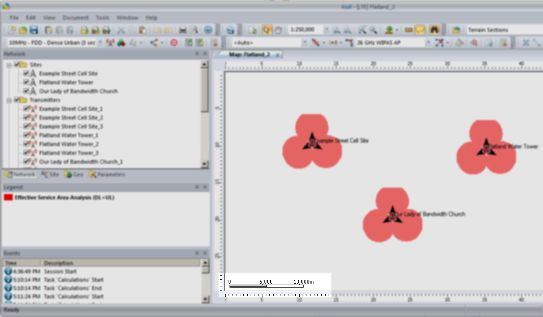
But if we have a look at the scale in the bottom left of the screen that’s understandable, our sites are ~10km apart…
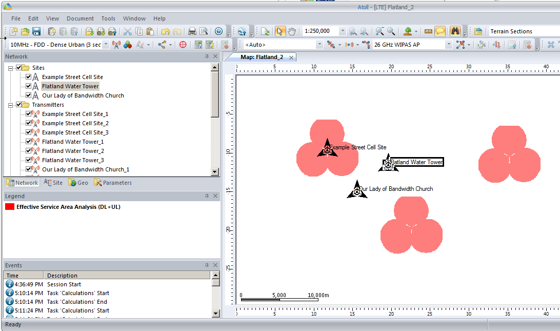
So let’s cheat a little by clicking and dragging on each cell site to bring them closer together, in real life we can’t move sites quite so easily…
You’ll notice our prediction hasn’t changed, so let’s recalculate that by right clicking on our Prediction and selecting Calculate again,
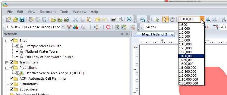
We’ll also set our zoom level from 1:250,000 to something a bit more reasonable like 1:100,000
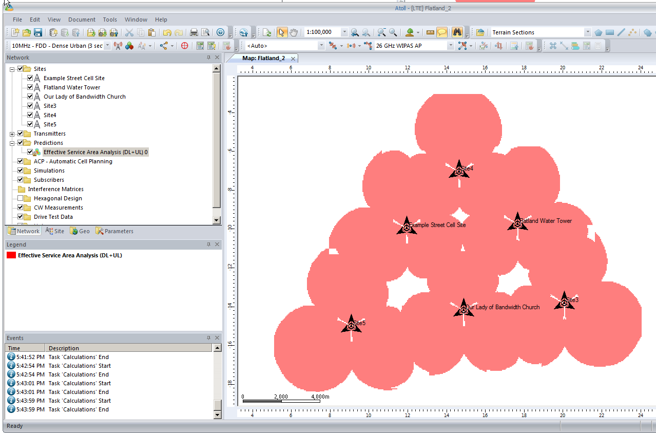
So now our 3 sites have got one area fairly well covered, let’s throw in a few more sites to expand our footprint a bit.
We’ll add extra sites as we did at the start, and fill in those coverage gaps.
After we’ve added some extra sites we’ll recalculate our Coverage Predictions and have a look at how we’ve done.
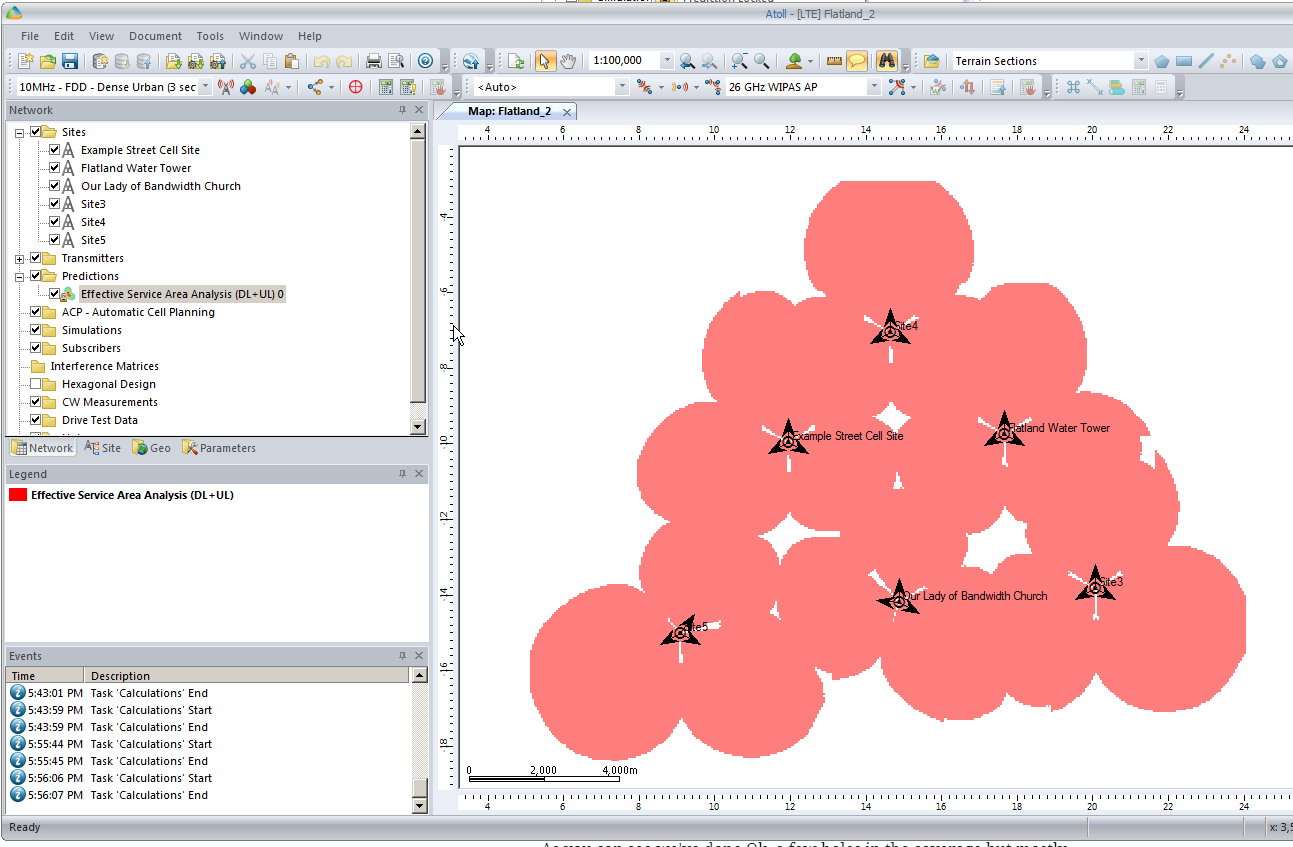
As you can see we’ve done Ok, a few holes in the coverage but mostly covered.
So next let’s do some tweaking to try and increase our predicted coverage,
By clicking on a site’s sector we can reorient the antenna to a different angle, by recalculating the coverage prediction we can see how this effects the predicted coverage.
By now you’ve probably got an idea of the basics of what we’re doing in Atoll, how changing the location, orientation and height of cells / sites affects the coverage, and how you can predict coverage.
In the upcoming posts we’ll cover adding real world data to Atoll so we can accurately model and predict how our RAN will perform.
We’ll look at how we can use Automatic Cell Planning to get the most optimal setup in terms of power settings, antenna orientations and tilts, etc for our existing sites.
We’ll be able to simulate subscribers, traffic flow, backhaul, and model our network all before a single truck rolls.
So stick around, the next post will be coming soon and will cover adding environment data.
In our last post we talked about getting our geospatial data right, and in our first post we covered the basics of adding sites and transmitters.
There’s a bit of a chicken-and-egg problem with site placement, antenna orientation, type and down-tilt.
If all our sites were populated and in place, we could look at optimizing coverage by changing azimuths / orientations, plug in our data and run some predictions / modeling and coming up with some solutions. Likewise if we’ve already done that we might want to calculate ideal down-tilt angles to get the most out of network.
But we’ve got no sites, no transmitters and no coverage predictions yet, so we’re probably going to need to ask ourselves a more basic, but harder question: Where will we put the cell sites?
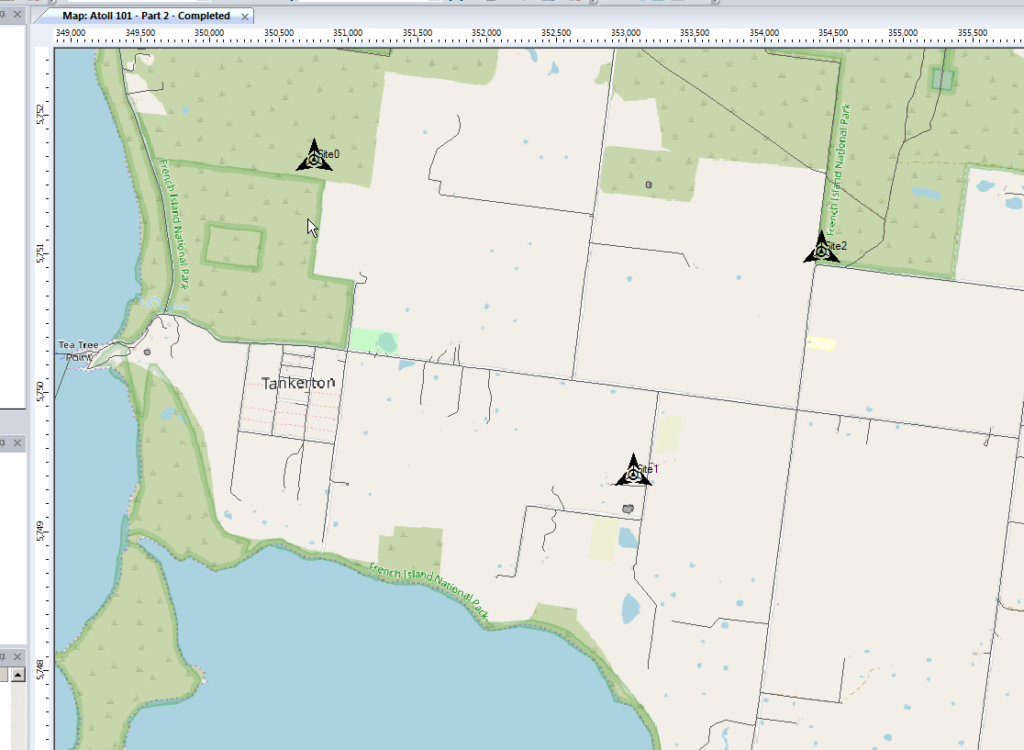
To keep this easy we’ll focus on providing the South Western corner of the Island, a town called Tankerton, with only 3 cell sites.
Manual Site Selection
In the very first post we put up a few sites, we’ll do the same, let’s place 3 sites in the bottom right of the island and attempt to provide contiguous coverage for the town with them;
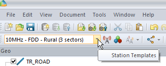
We’ll pick our Station Template and set it to FDD Rural as this is pretty remote.
Next we’ll add some sites and transmitters:
Click to place it on the map and add our cell sites;
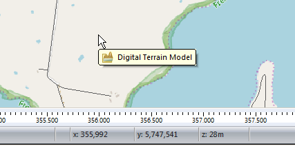
When we’re looking at where to place it, it’s good to remember that height (elevation) is good (To an extent), so when looking at where to place sites, keep an eye on the Z (Height) value in the bottom right, and try and pick sites with a good elevation.
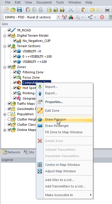
Setting Computation Zone
As we’re only focusing on a small part of the island we’ll set a Computation Zone to limit the calculations / computations Atoll has to do to a set region.
I’ve chosen to draw a Polygon around the area, but you could also just get away with drawing a Rectangle, around the area we’re interested in.
This just constrains everything so we’re only crunching numbers inside that area.
Predictions
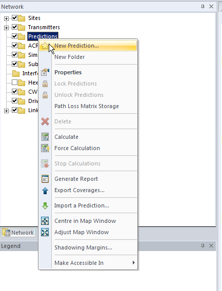
So now we’ve put our 3 sites out & constrained to the Tankerton area, let’s see how much of the area we’ve covered, we’ll jump to the Network tab, right click on Predictions and select New Prediction
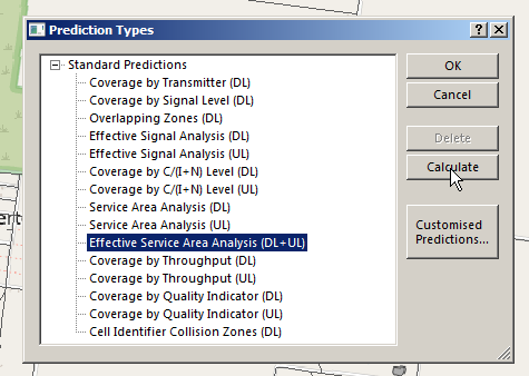
There’s a lot of predictions we can run, but we’ll go simple and select Effective Service Area Analysis (UL + DL) & click Calculate
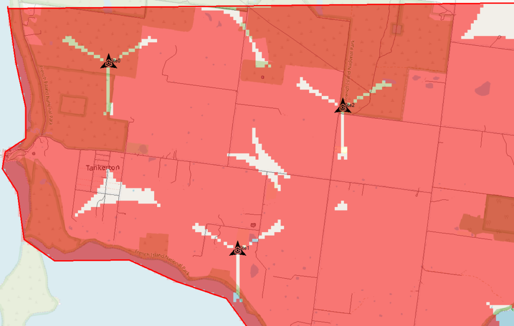
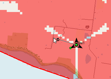
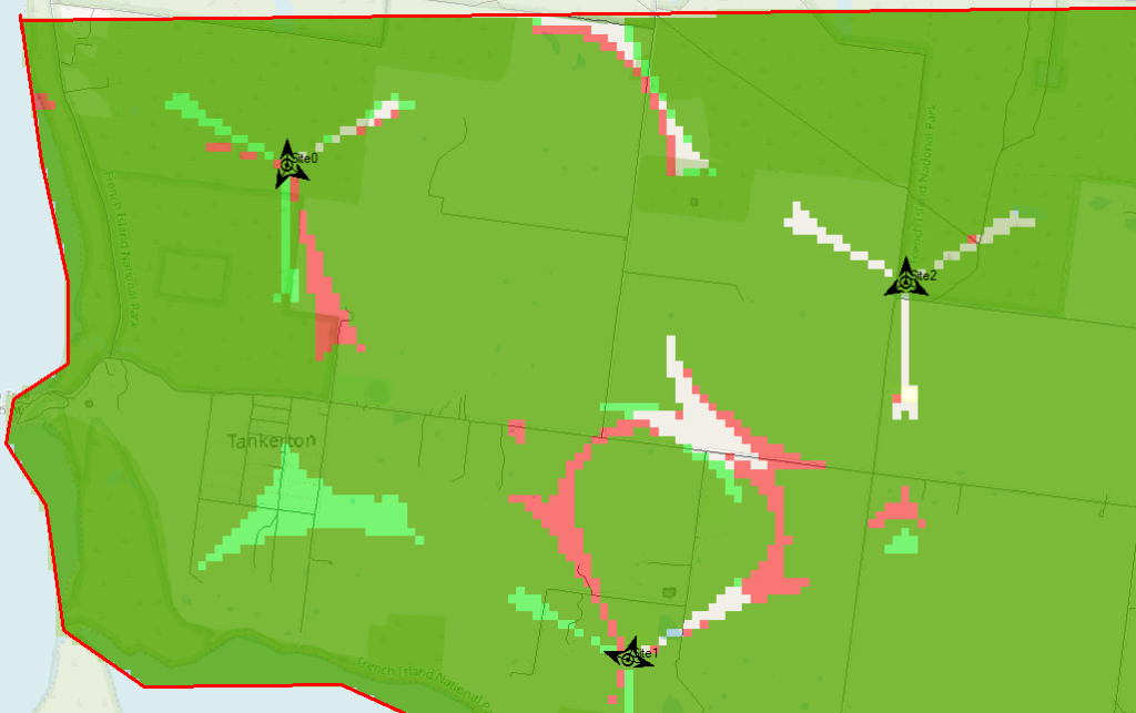
Atoll will crunch the numbers and give us a simple overlay, showing the areas with and without coverage.
The areas in red are predicted to have coverage, and the areas with no shading will be our blackspots / “notspots”.
We’ve covered most of the area, but we can improve.
Manually Tweaking Attributes
So there’s still some holes in our coverage, so let’s adjust the azimuth of some of the antennas and see if we can fill them.
Click on each of the arrows on the site, each of these represents an antenna / cell and we can change the angles.
So after a bit of fiddling I think I’ve got a better antenna azimuth for each of the sectors on each of my 3 sites.
Let’s compare that to what we had before to see if we’ve made it better or worse,
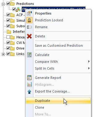
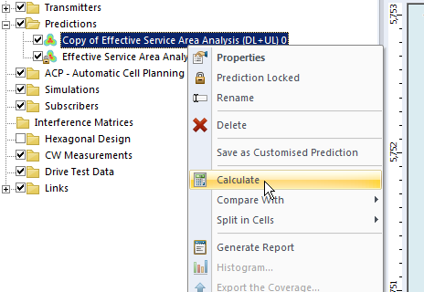
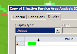
We’ll Duplicate the Effective Service Area Analysis prediction we created before & calculate it.
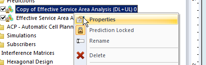
To make viewing a bit easier we’ll edit the properties of the copy and set it to a different colour:
Now I can see at a glance how much better we’re looking;
The obvious problem here is I could tweak and tweak and improve some things, make others worse, and we’d be here forever.
Luckily Atoll can do a better job of fiddling with each parameter for us and selecting the configuration that leads to the best performance in our RAN.
Automatic Cell Planning
Enter Automatic Cell Planning, to adjust the parameters we set to find the most optimal setup,
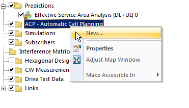
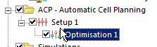
We’ll right click on ACP – Automatic Cell Planning and create a new one.
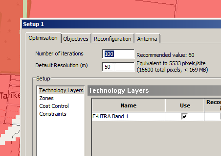
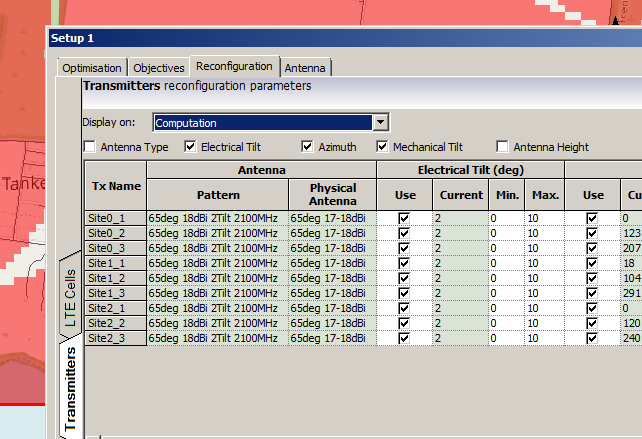
From here we set how many iterations we want to try out (more leads to better results but takes longer to compute), the parameters we want to change (ie Azimuth, Tilt, Antenna type, etc).
Setting number of iterations – Higher leads to better results but takes longer to calculate and has diminishing returnsWe’ll allow the Tilt (Electrical & Mechanical) to be adjusted as well as the Azimuth of each antenna.
When you’ve set the parameters you want, click Run and Atoll will start running through possible parameter combinations and measuring how they perform.
Once it’s run you’ll be able to view the Optomization
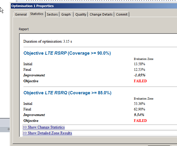
The report shows you the results, improvements in RSSI and RSSQ;
Here we can see we boosted the RSRQ (The quality of the signal) by 9.5%, but had to sacrifice RSRP (Signal power) by 1%.
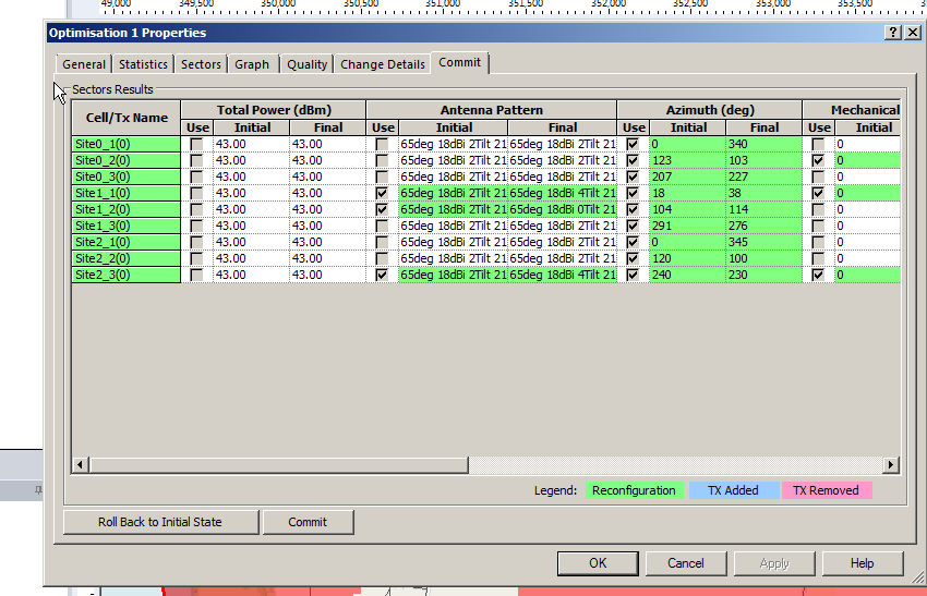
Sacrificies have to be made, and if you’re happy with this you can view the details of the changes, and commit the adjustments.
Committing the changes adjusts all the Transmitters in the area to the listed values, after which we can run our Predictions again to compare like we did earlier.
So that’s what we’ve got when we randomly place sites, we can use Atoll to optomize what we’ve already got, but what if we left the picking of cell sites up to Atoll to look for better options?
In our next post we’ll look at Site Selection using ACP, and constraining it. This means we can tell Atoll to just find the best sites, or load in a list of possible sites and let Atoll determine which are the best candidates.