As our subscribers are mobile, moving between base stations / cells, the destination of the incoming GTP-U packets needs to be updated every time the subscriber moves from one cell to another.
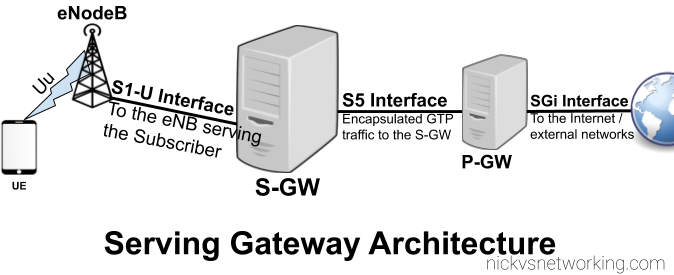
As we covered in the last post, the Packet Gateway (P-GW) handles decapsulating and encapsulating this traffic into GTP from external networks, and vise-versa. The Packet Gateway sends the traffic onto a Serving Gateway, that forwards the GTP-U traffic onto the eNodeB serving the user.
So why not just route the traffic from the Packet Gateway directly to the eNodeB?
As our users are inherently mobile, the signalling load to keep updating the destination of the incoming GTP-U traffic to the correct eNB, would put an immense load on the P-GW. So an intermediary gateway – the Serving Gateway (S-GW), is introduced.
The S-GW handles the mobility between cells, and takes the load of the P-GW. The P-GW just hands the traffic to a S-GW and let’s the S-GW handle the mobility.
It’s worth keeping in mind that most LTE connections are not “always on”. Subscribers (UEs) go into “Idle Mode”, in which the data connection and the radio connection is essentially paused, and able to be bought back at a moments notice (this allows us to get better battery life on the UE and better frequency utilisation).
When a user enters Idle Mode, an incoming packet needs to be buffered until the Subscriber/UE can get paged and come back online. Again this function is handled by the S-GW; buffering packets until the UE comes available then forwarding them on.
Most people think of SIP when it comes to FreeSWITCH, Asterisk and Kamailio, but all three support WebRTC.
FreeSWITCH makes WebRTC fairly easy to use and treats it much the same way as any SIP endpoint, in terms of registration and diaplan.
Setting up the SIP Profile
On the SIP profile we’ll need to activate WebRTC you’ll need to ensure a few lines of config are present:
    <!-- for sip over secure websocket support -->
    <!-- You need wss.pem in $${certs_dir} for wss or one will be created for you -->
    <param name="wss-binding" value=":7443"/>
Next you’ll need to restart FreeSWITCH and a self-signed certificate should get loaded,
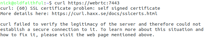
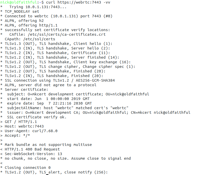
Once you’ve restarted FreeSWITCH will fail to detect any WebSocket certificate and generate a self signed certificate for you. This means that you can verify FreeSWITCH is listening as expected using Curl:
curl https://yourhostname:7443 -vvv
You should see an error regarding the connection failing due to an invalid certificate, if so, great! Let’s put in a valid certificate.
If not double check the firewall on your server allow traffic to port TCP 7443,
Loading your TLS Certificate
WebRTC & websocket are recent standards – this means a valid TLS certificate is mandatory. So to get this to work you’ll need a valid SSL certificate.
When we restarted FreeSWITCH after adding the wss-binding config a certificate was automatically generated in the $${certs_dir} of FreeSWITCH,
You can verify where the certs_dir is by echoing out the variable in FreeSWITCH:
fs_cli -x 'eval $${certs_dir}'
Unless you’ve changed it you’ll probably find your certs in /etc/freeswitch/tls/
The certificate and private key are stored in a single file, with the Certificate and the Private Key appended to the end,
In my case the certificate is called “webrtc.pem” and the private key file is “webrtc-key.pem”,
I’ll need to start by replacing the contents of the current certificate/ key file wss.pem with the certificate I’ve got webrtc.pem, and then appending the private key – webrtc-key.pem to the end of wss.pem,
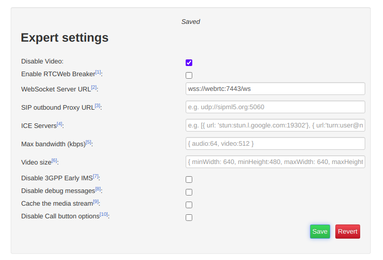
We’ll start by clicking the “Export Mode” button to set our wss:// URL;
Change the WebSocket Server URL to the URL of your FreeSWITCH instance (you must use a domain, not an IP Address)
If you’re running behind a NAT adding ICE servers is probably a good idea, although this will slow down connection times, you can use Google’s public STUN server by pasting in the below value:
[{ url: 'stun:stun.l.google.com:19302'}]
Finally we’ll save those settings and return back to the main tab,
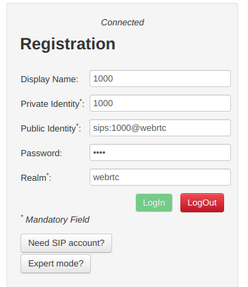
You’ll need to register with a username and password that’s valid on the FreeSWITCH box, in my case I’m using 1000 with the password 1000 (exists by default),
Replace webrtc with the domain name of your FreeSWITCH instance,
Finally you should be able to click Login and see Connected above,
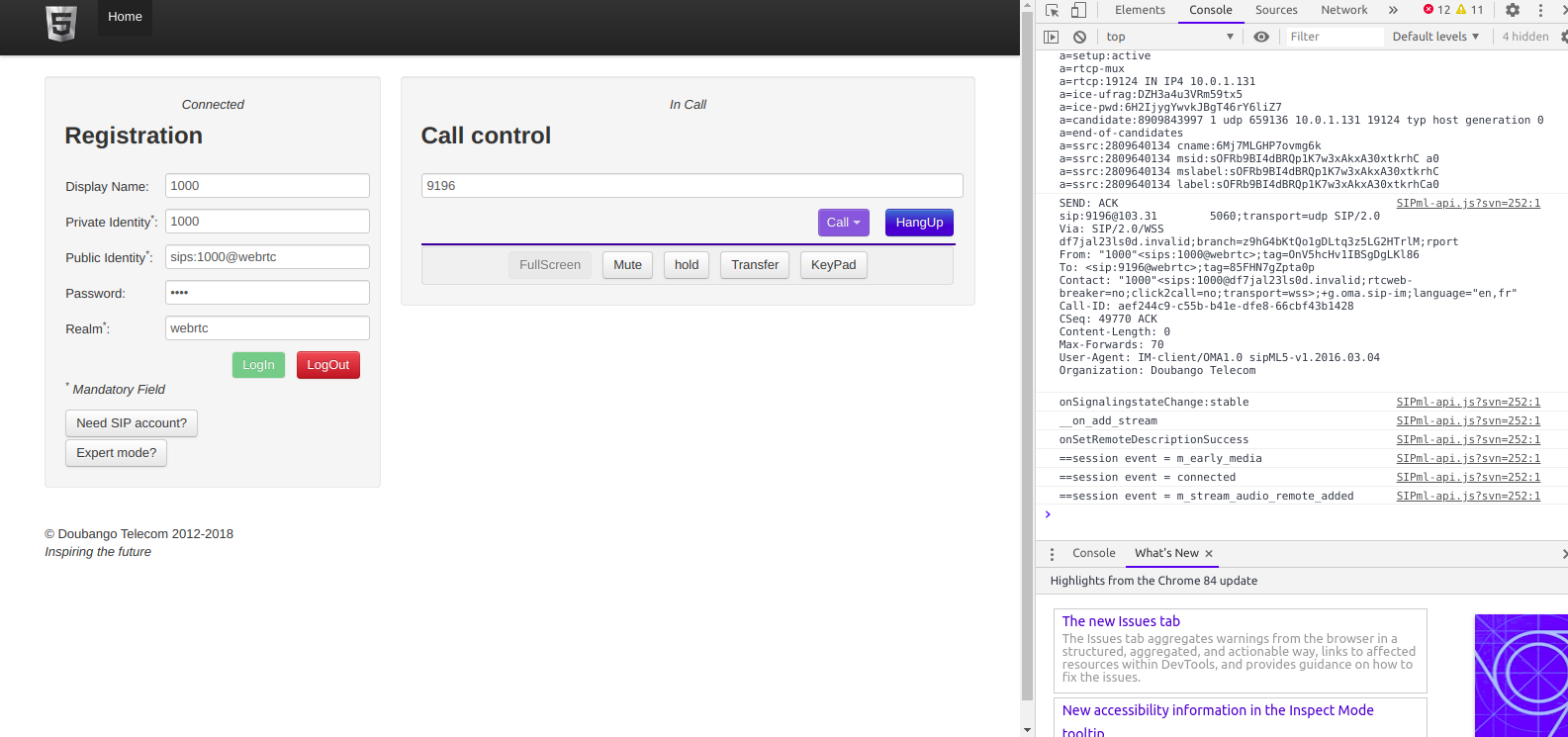
Then we can make calls to endpoints on FreeSWITCH using the dial box;
The Debug console in your browser will provide all the info you need to debug any issues, and you can trace WebSocket traffic using Sofia like any other SIP traffic.
Hopefully this was useful to you – I’ll cover more of WebRTC on Asterisk and also Kamailio in later posts!
It’s a seemingly simple question, the answer to which is – however you want, sorry if that’s not a simple answer.
I’ve talked about the strengths and weaknesses of Kamailio and Asterisk in my post Kamailio vs Asterisk, so how about we use them to work together?
The State of Play
So before we go into the nitty gritty, let’s imagine we’ve got an Asterisk box with a call queue with Alice and Bob in it, set to ring those users if they’re not already on a call.
Each time a call comes in, Asterisk looks at who in the queue is not already on a call, and rings their phone.
Now let’s imagine we’re facing a scenario where the single Asterisk box we’ve got is struggling, and we want to add a second to share the load.
We do it, and now we’ve got two Asterisk boxes and a Kamailio load balancer to split the traffic between the two boxes.
Now each time a call comes in, Kamailio sends the SIP INVITE to one of the two Asterisk boxes, and when it does, that Asterisk box looks at who is in the queue and not already on a call, and then rings their phone.
Let’s imagine a scenario where a Alice & Bob are both on calls on Asterisk box A, and another call comes in this call is routed to Asterisk box B. Asterisk box B looks at who is in the queue and who is already on a call, the problem is Alice and Bob are on calls on Asterisk box A, so Asterisk box B doesn’t know they’re both on a call and tries to ring them.
We have a problem.
Scaling stateful apps is a real headache,
So have a good long hard think about how to handle these issues before going down this path!
Oftentimes I’m developing something locally and I need an SSL Certificate.
I’m too cheap to buy a valid SSL cert for a subdomain like “dev.nickvsnetworking.com” and often the domain changes based on what I’m doing,
LetsEncrypt is great, but requires your server to be public facing and be a web server, which for dev stuff isn’t really practical,
Enter mkcert – a tool that allows you to generate valid SSL certificates on your machine for any domain, the catch is that it’s only on your machine.
I’m working on a WebSocket platform at the moment, which requires an SSL certificate.
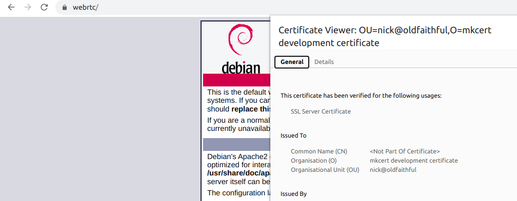
So I set an entry in my hosts file to point “webrtc” to the IP of one of the machines,
I then generated the cert on my local machine,
mkcert -install webrtc
Which outputs the certificate and private key, which I copied it onto the server I’m working on, twiddled some knobs in Apache2 and presto, valid cert!
The downside is of course anyone else going to this site would see the cert as invalid, but as it’s just me, it doesn’t matter!
A question that seems to come up often, is how to provide a static IPs to UEs on Open5GS EPC.
By default all UEs are allocated an internal IP that the server the P-GW is running on NATs out, but many users want to avoid NAT, for obvious reasons.
Open5GS has the ability to set a Static IP for each APN a subscriber has, but let’s get one thing out of the way first;
LTE is not Ethernet. No broadcast, no multicast. Each IP Address is best thought of as a single /32 network. This means you can’t have the UEs in your LTE network in the same 192.168.1.x subnet as your home network along with your laptop and printer, it’s not how it works.
So with that out of the way, let’s talk about how to do static IP address allocation in Open5GS EPC.
Assigning a Subscriber a Static IP Address
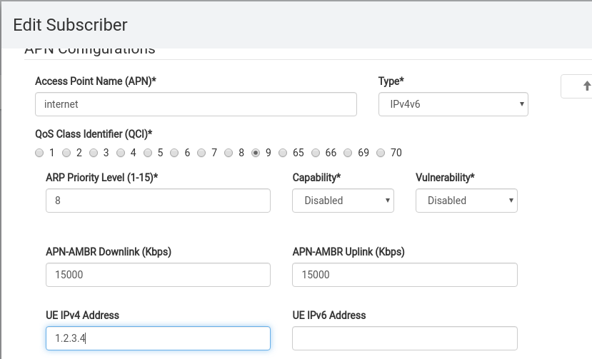
From the HSS edit the Subscriber and in the UE IPv4 or UE IPv6 address, set the static address you want to use.
You can set any UE IP Address here and it’ll get allocated to that UE.
But – there’s an issue.
The problem is not so much on the Open5GS P-GW implementation, but just how TCP/IP routing works in general.
Let’s say I assign the UE IPv4 address 1.2.3.4 to my UE. From the UE it sends a packet with the IPv4 Source address of 1.2.3.4 to anywhere on the internet, the eNB puts the packet in GTP and eventually the it gets to the P-GW which sends it out onto the internet from the source address 1.2.3.4.
The problem is that the response will never get back to me, as 1.2.3.4 is not allocated to me and will never make it back to my P-GW, so never relayed back to the UE.
For TCP traffic this means I can send the SYN with the source address of 1.2.3.4, but the SYN/ACK will be routed back to the real 1.2.3.4, and not to me, so the TCP socket will never get opened.
So while we can set a static IPs to be allocated to UEs in Open5GS, unless the traffic can be routed back to these IPs it’s not much use.
Routing
So let’s say we have assigned IP 1.2.3.4 to the UE, we’d need to put a static route on our routers to route traffic to the IP of the PGW. In my case the PGW is 10.0.1.121, so I’ll need to add a static route to get traffic destined 1.2.3.4/32 to 10.0.1.121.
In a more common case we’d assign internal IP subnets for the UE pool, and then add routes for the entire subnet to the IP of the PGW.
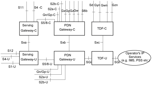
3GPP release 14 introduced the concept of CUPS – Control & User Plane Separation, and the Sx interface, this allows the control plane (GTP-C) functionality and the user plane (GTP-U) functionality to be separated, and run in a distributed fashion, allowing the node a user’s GTP-U traffic flows through to be in a different location to where the Control / Signalling traffic (GTP-C) flows.
In practice that means for an LTE EPC this means we split our P-GW and S-GW into a minimum of two network elements each.
A P-GW is split and becomes a P-GW-C that handles the P-GW Control Plane traffic (GTPv2-C) and a P-GW-U speaking GTP-U for our User Plane traffic. But the split doesn’t need to stop there, one P-GW-C could control multiple P-GW-Us, routing the user plane traffic. Sames goes for S-GW being split into S-GW-C and S-GW-U,
This would mean we could have a P-GW-U located closer to a eNB / User to reduce latency, by allowing GTP-U traffic to break out on a node closer to the user.
It also means we can scale better too, if we need to handle more data traffic, but not necessarily more control plane traffic, we can just add more P-GW-U nodes to handle this.
To manage this a new protocol was defined – PFCP – the Packet Forwarding Control Protocol. For LTE this is refereed to as the Sx reference point, it’ also reused in 5G-SA as the N4 reference point.
When a GTP-C “Create Session Request” comes into a P-GW for example from an S-GW, a PFCP “Session Establishment Request” is sent by the P-GW-C to the P-GW-U with much the same information that was in the GTP-C request, to setup the session.
So why split the Control and User Plane traffic if you’re going to just relay the GTP-C traffic in a different format?
That was my first question – the answer is that keeping the GTP-C interface ensures backward compatibility with older MMEs, PCRFs, charging systems, and allows a staged roll out and bolting on extra capacity.
GTP-C disappears entirely in 5G Standalone architecture and is replaced with the N4 interface, which uses PFCP for the Control Plan and GTP-U again.
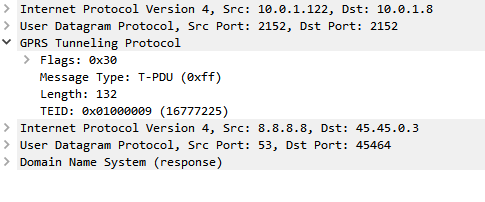
Here’s a capture from Open5Gs core showing GTPv2C and PFCP in play.
Recently, ACMA / Communications Alliance updated the rules defining cabling – S009 – “Installation requirements for customer cabling” aka the “Wiring Rules” or “Cabling Bible”.
I don’t talk much about cabling on this blog – but I’m still a registered cabler so need to keep up to date on the changes, and quite a lot has changed since the last update in 2013 – Authority to Alter (A2A) has moved from Telstra to NBNco, PayTV over HFC is far less common, and the NBN rollout is “finished”.
So what are the key changes I need to know about? I had a read and compared to S009 / 2013, and here are they are:
“Supervised” Definition
In order to gain cabling registration you need 360 hours of supervised cabling experience. The specification has been updated to define exactly what supervised means,
4.2.59 instructed person a person instructed or supervised by a Skilled Person as to energy sources and who can responsibly use equipment safeguards and precautionary safeguards with respect to those energy sources. Note: Supervised, as used in the definition, means having the direction and oversight of the performance of others.
ES3 (Electrical energy source class 3 (ES3)) Definition & Rules
Reverse power feed, used in NBN FTTC tech, as well as higher voltages used for EWIS and PA systems, has led to the introduction of a new classification – ES3, for cabling that exceeds the ES2 limits,
a metallic circuit utilised for communications or Power Feeding, or both, that— (a) exceeds the ES2 voltage and touch current limits; (b) does not exceed 400 V d.c. between conductors; and (c) does not exceed current as specified in AS/NZS 11801.1 or ISO/IEC 11801-1.
4.2.45 ES3 generic circuit
ES3 falls into two categories, which specific whether it can be carried over generic cabling or not,
(a) over Generic Cabling, in this Standard, are based on— (i) circuit voltage not exceeding 400 V d.c. between conductors; and (ii) circuit current not exceeding that specified in AS/NZS 11801.1 or ISO/IEC 11801-1. Where voltages and currents exceed these limits, then Special Application Cabling, as classified in Item F.2(b), should be used. (b) over Special Application Cabling in this Standard, are based on a voltage limit and current limit set by Cable manufacturer for the specific Cable and its installation requirements
F.2
So if part a is exceeded, Special Application cabling is required;
the cabling must meet a higher standard defined for ES3
must be identified by it’s sheath colour and markings at regular intervals
cabling has to be separated from other services (sub-ducted or separated by a barrier or more than 150mm)
must carry a warning label wherever the conductive part of the circuit is exposed (frames / joints) stating it is an ES3 service
service may not be terminated on a plug if the plug may have exposed contacts (requires a plug / socket with shutters)
an equipment circuit within the ICT Network not connected to Mains power, intended to supply or receive DC power at voltages exceeding the limits of ES2, and on which transient overvoltages or overcurrents may occur.
4.2.85
Examples are PoE, ring current, USB-C / USB3, etc.
RFT circuits are classified as ES3 circuits and subject to the same conditions.
New Conductor Size / Temperature Recommendations
S009 / 2013 did not specific recommended (not mandated) size & temperature rating for generic cabling / jumpering.
It comes down to:
“have a maximum conductor resistance of 0.0938 Ω/m at 20° C “ and “the cable should not be installed in a manner that may cause the maximum operating temperature rating of the Cable to be exceeded.”
5.6.2
Plug Terminated Cabling Requirements
Moveable cabling / plug terminated cabling must not be used unless:
the Plug is an integral part of a device that is fastened to a wall, floor or ceiling or other permanent building element; or (b) the Plug is not fixed and— (i) the Plug terminates a section of Movable Cabling; (ii) the Plug is to mate with a Port on an item of fixed Customer Equipment; and (iii) in every position to which it may be moved when the Plug is not mated with the Port, every part of the section of Movable Cabling is either out of Arm’s Reach or housed in a Secure Enclosure that is fastened to a wall, floor or ceiling or other permanent building element.
5.9.1
Network Boundary Definition Update
A new Appendix (J) has been added with updated (informative only) definitions of Network Boundaries with examples, to support all the new network boundary definitions introduced with the access technology mix(fibre, HFC and wireless terminations).
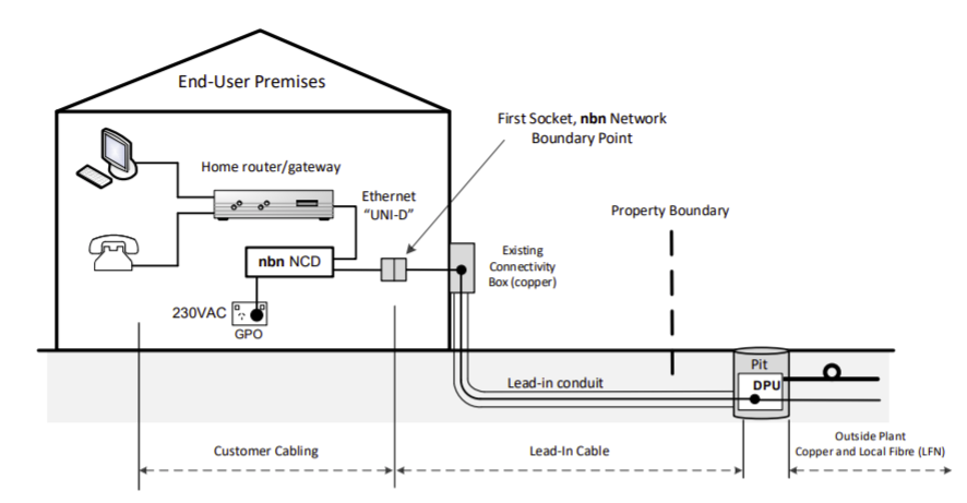
FTTC Deployment Information (Informative)
A new Appendix (O) has been added providing information in regards to FTTC and it’s requirement to isolate the first socket from the rest of the cabling – Something that in practice seems to be a rarity.
Labelling & Safety Rules for Fibre Optic Cabling
A new requirement has been added to 11.1 in regards to Fibre Optic cabling must:
Have a Warning of potential hazardous laser levels
Have a warning regarding Access to emitted radiation
Types of laser warning markings
Laser warning marking style
Laser explanatory label wording
Marking durability of labels
Fibre outlets in work areas are except
Groups of optical fibre connectors may be marked as a group
Multiple markings – ie one inside the container one outside
Unused optical fibre connectors and adaptors must be covered
The S1 interface can be pretty noisy, which makes it hard to find the info you’re looking for.
So how do we find all the packets relating to a single subscriber / IMSI amidst a sea of S1 packets?
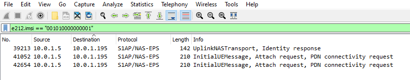
The S1 interface only contains the IMSI in certain NAS messages, so the first step in tracing a subscriber is to find the initial attach request from that subscriber containing the IMSI.
Luckily we can filter in Wireshark to find the IMSI we’re after;
Quick note – Not all IntialUEMessages will contain the IMSI – If the subscriber has already established comms with the MME it’ll instead be using a temporary identifier – M-TMSI, unless you’ve got a way to see the M-TMSI -> IMSI mapping on the MME you’ll be out of luck.
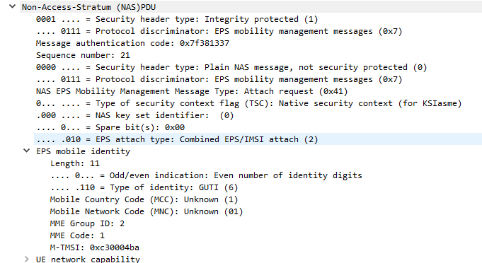
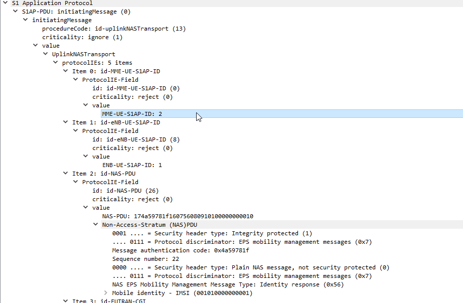
Next up let’s take a look at the contents of one of these packets,
Inside the protocolIEs is the MME_UE_S1AP_ID – This unique identifier will identify all S1 signalling for a single user.
The MME_UE_S1AP_ID is a unique identifier, assigned by the MME to identify which signaling messages are for which subscriber.
(It’s worth noting the MME_UE_S1AP_ID is only unique to the MME – If you’ve got multiple MMEs the same MME_UE_S1AP_ID could be assigned by each).
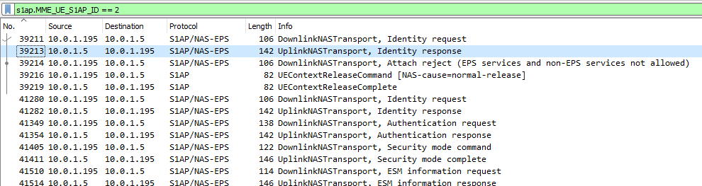
So now we have the MME_UE_S1AP_ID, we can filter all S1 messaging containing that MME_UE_S1AP_ID, we’ll use this Wireshark filter to get it:
s1ap.MME_UE_S1AP_ID == 2
Boom, there’s a all the signalling for that subscriber.
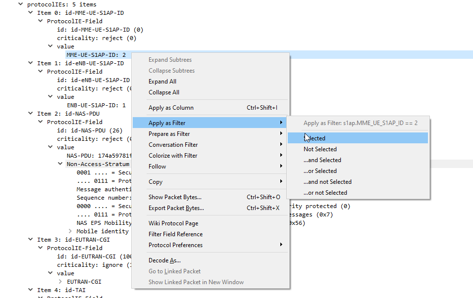
Alternatively you can just right click on the value and apply it as a filter instead of typing everything in,
Hopefully that’ll help you filter to find what you’re looking for!
So a problem had arisen, carriers wanted to change certain carrier related settings on devices (Specifically the Carrier Config Manager) in the Android ecosystem. The Android maintainers didn’t want to open the permissions to change these settings to everyone, only the carrier providing service to that device.
And if you purchased a phone from Carrier A, and moved to Carrier B, how do you manage the permissions for Carrier B’s app and then restrict Carrier A’s app?
The carrier loads a certificate onto the SIM Cards, and signing Android Apps with this certificate, allowing the Android OS to verify the certificate on the card and the App are known to each other, and thus the carrier issuing the SIM card also issued the app, and presto, the permissions are granted to the app.
Carriers have full control of the UICC, so this mechanism provides a secure and flexible way to manage apps from the mobile network operator (MNO) hosted on generic app distribution channels (such as Google Play) while retaining special privileges on devices and without the need to sign apps with the per-device platform certificate or preinstall as a system app.
If you’re using an GSM / GPRS, UMTS, LTE or NR network, there’s a good chance all your data to and from the terminal is encapsulated in GTP.
GTP encapsulates user’s data into a GTP PDU / packet that can be redirected easily. This means as users of the network roam around from one part of the network to another, the destination IP of the GTP tunnel just needs to be updated, but the user’s IP address doesn’t change for the duration of their session as the user’s data is in the GTP payload.
One thing that’s a bit confusing is the TEID – Tunnel Endpoint Identifier.
Each tunnel has a sender TEID and transmitter TEID pair, as setup in the Create Session Request / Create Session Response, but in our GTP packet we only see one TEID.
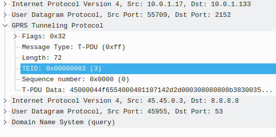
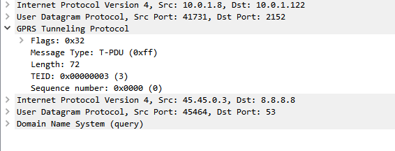
There’s not much to a GTP-U header; at 8 bytes in all it’s pretty lightweight. Flags, message type and length are all pretty self explanatory. There’s an optional sequence number, the TEID value and the payload itself.
So the TEID identifies the tunnel, but it’s worth keeping in mind that the TEID only identifies a data flow from one Network Element to another, for example eNB to S-GW would have one TEID, while S-GW to P-GW would have another TEID.
Each tunnel has two TEIDs, a sending TEID and a receiving TEID. For some reason (Minimize overhead on backhaul maybe?) only the sender TEID is included in the GTP header;
This means a packet that’s coming from a mobile / UE will have one TEID, while a packet that’s going to the same mobile / UE will have a different TEID.
Mapping out TIEDs is typically done by looking at the Create Session Request / Responses, the Create Session Request will have one TIED, while the Create Session Response will have a different TIED, thus giving you your TIED pair.
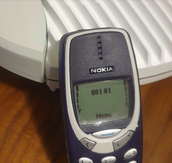
With just one cell/BTS, your mobile phone isn’t all that mobile.
So GSM has the concept of handovers – Once BTS (cell) can handover a call to another cell (BTS), thus allowing us to move between BTSs and keep talking on a call.
Note: I’ll use the term BTS here, because we’ve talked a lot about BTSs throughout this series. Technically a BTS can be made up of one or more cells, but to keep the language consistent with the rest of the posts I’ll use BTS, even though were talking about the cell of a BTS.
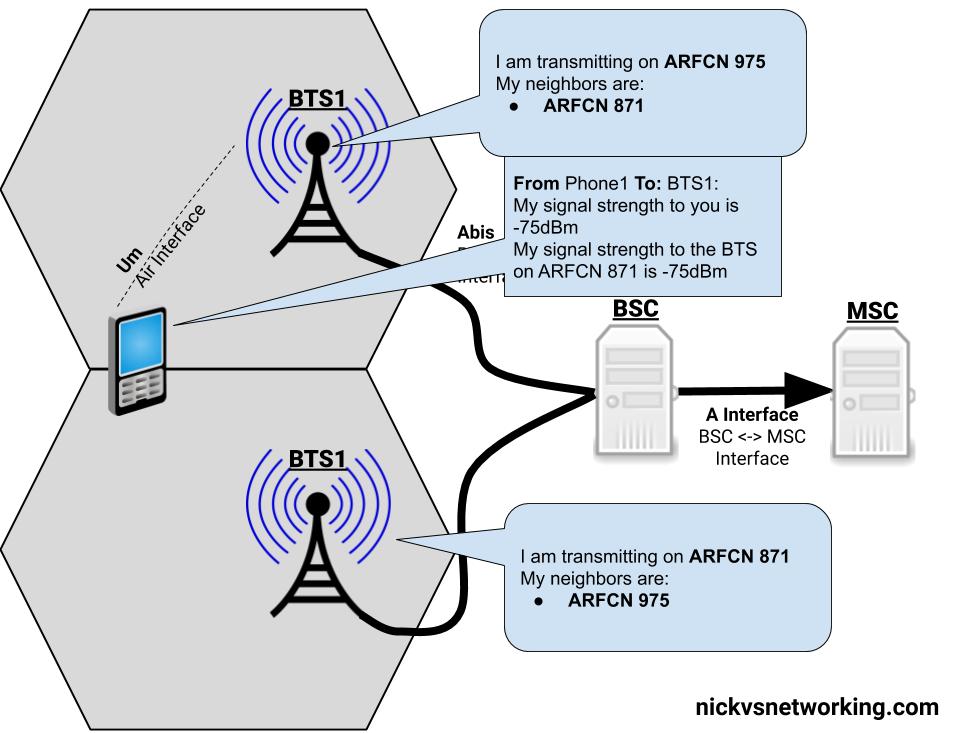
If we’re on a call, in an area served by BTS1, and we’re moving towards BTS2, at some point the signal strength from BTS2 will surpass the signal strength from BTS1, and the phone will be handed over from BTS1 to BTS2.
Handovers typically only occur when a channel is in use (ie on a phone call) if a phone isn’t in use, there’s no need to seamlessly handover as a brief loss of connectivity isn’t going to be noticed by the users.
Measurements
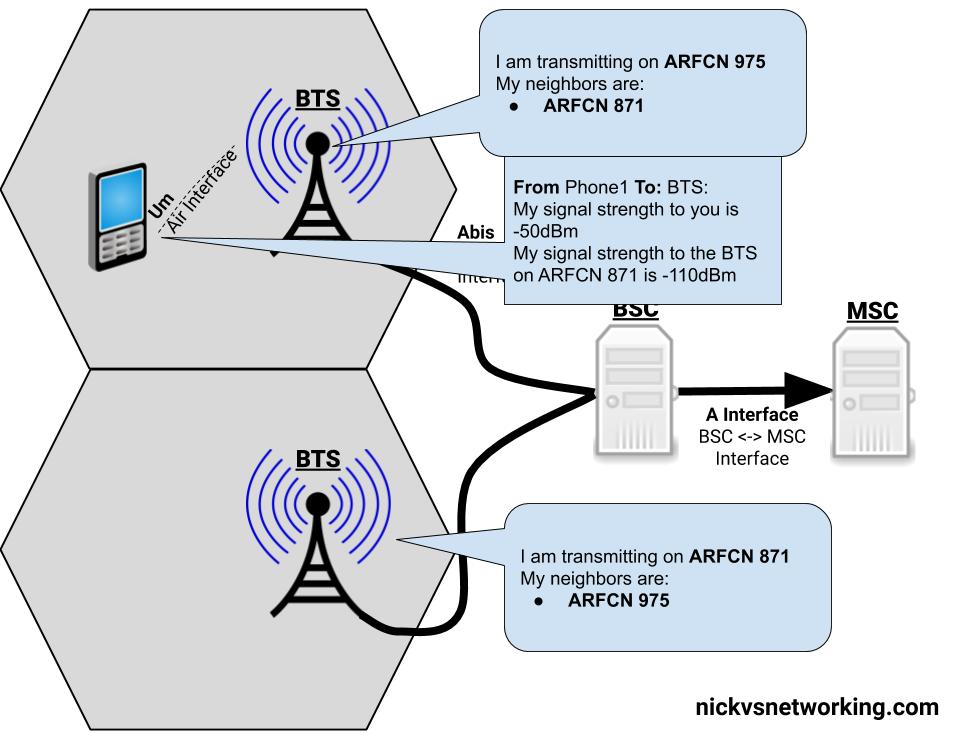
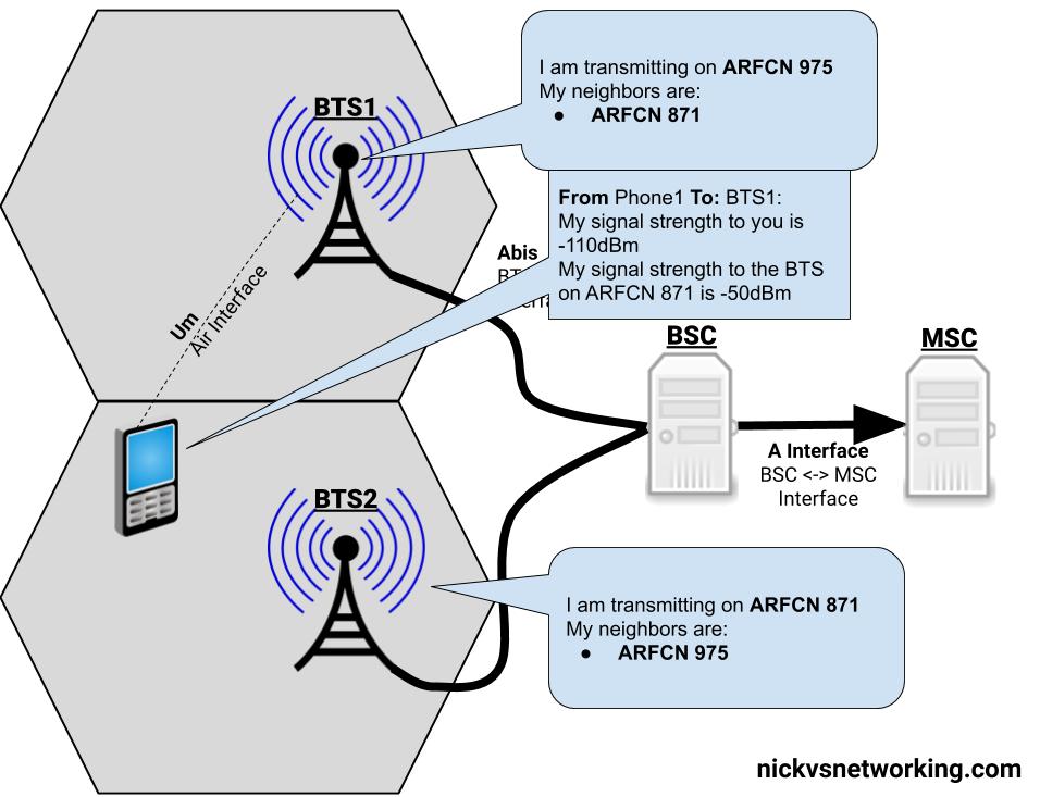
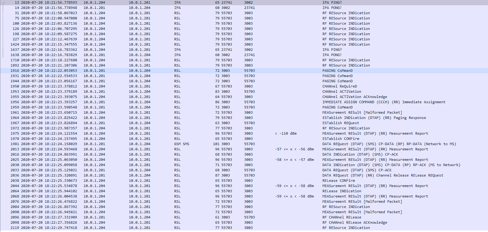
The question as to when to handover a call to a neighbouring cell, comes down to the signal strength levels the phone is experiencing.
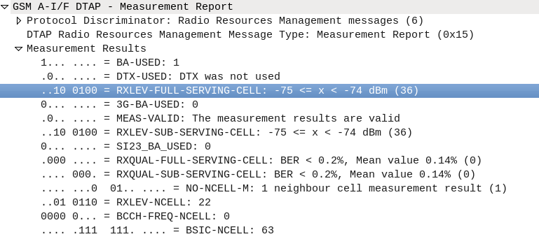
The phone measures the signal strength of up to 6 nearby (neighbouring) BTSs, and reports what signal strength it’s receiving to the BTS that’s currently serving it.
The BTS then sends this info to the BSC, in the RXLEV fields of a RSL Measurement Report packet.
RXLEV fields of a RSL Measurement Report packet.
With this information the BSC makes the determination of when to handover the call to a neighbouring BTS.
There’s a lot of parameters that the BSC takes into account when making the decision to handover to a neighbouring BTS, but for the purposes of this explanation, we’ll simplify this and just imagine it’s based on which BTS has the strongest signal strength as seen by the phone.
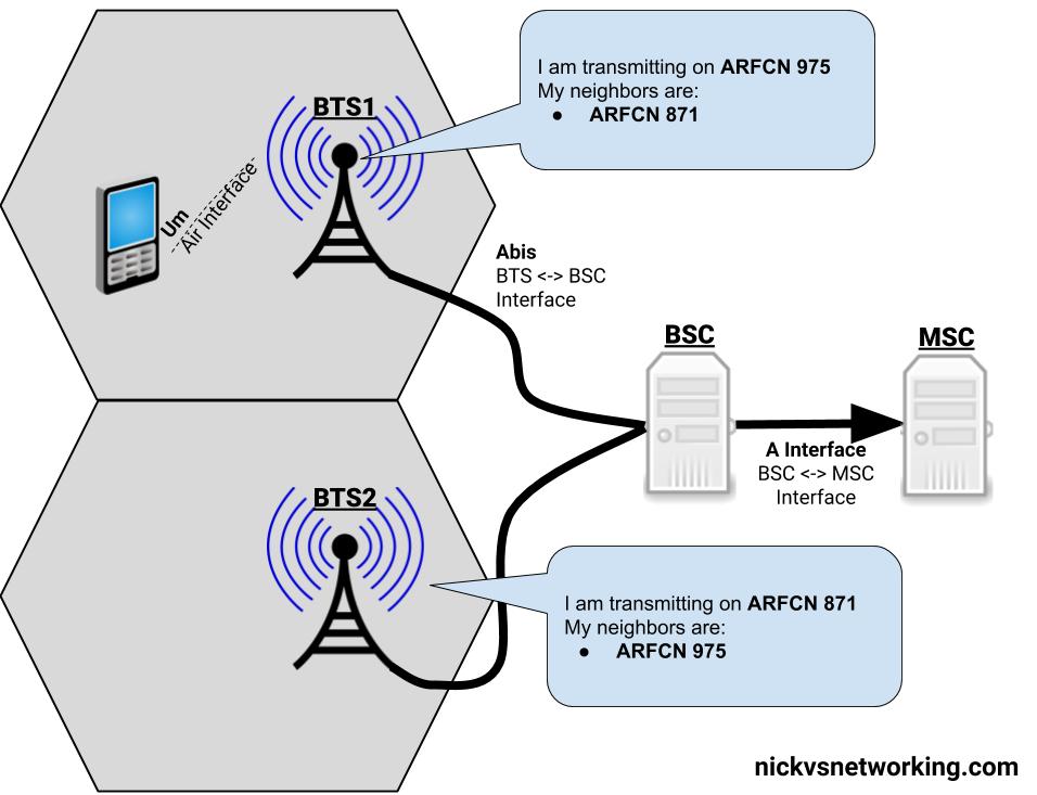
Everybody needs good Neighbors
Our phone can only monitor the signal strength of so many neighboring cells at once (Up to 6). So in order to know which frequency (known as ARFCNs) to take signal strength measurements on, our phone needs to know the frequencies it should expect to see neighbours, so it can measure these frequencies.
The System Information Block 2 is broadcast by the BTS on the BCCH and SACCH channels, and contains the ARFCNs (Frequencies) of the BTSs that neighbour that cell.
With this info our Phone only needs to monitor the frequencies (ARFCNs) of the cells nearby it’s been told about in the SIB2 to check the received power levels on those frequences.
The Handover
This is vastly simplified…
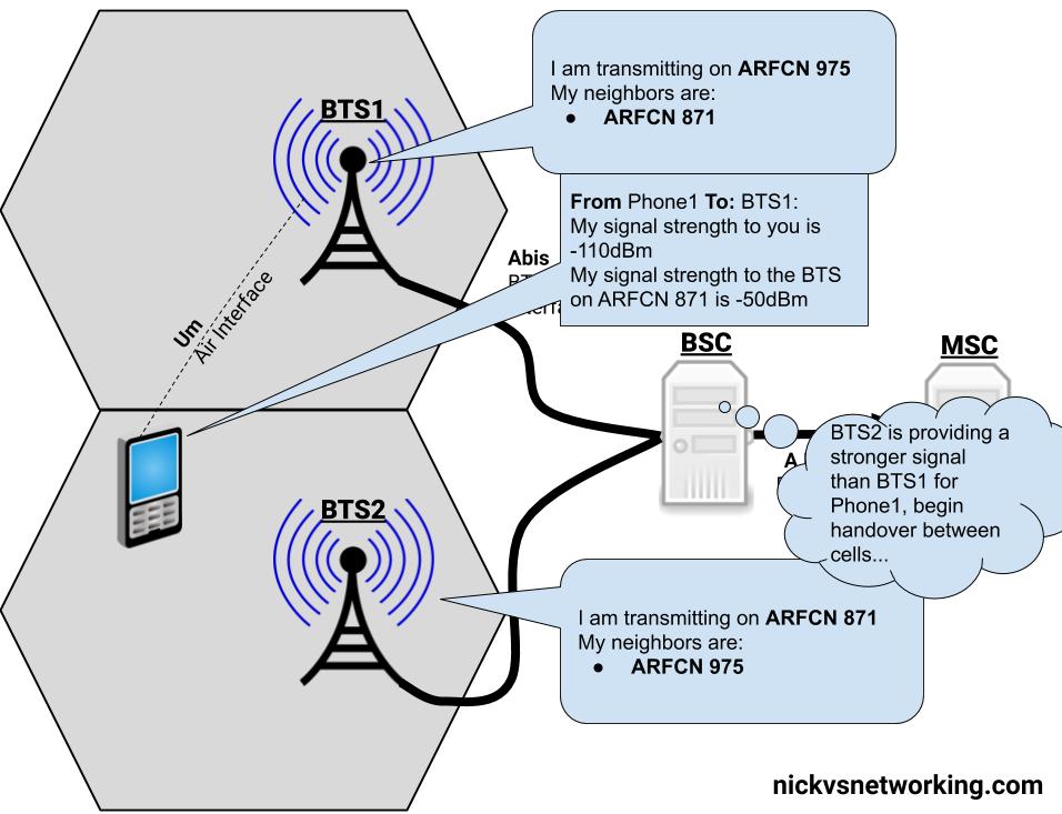
So our phone is armed with the list of neighbouring cell frequencies (ARFCNs) and it’s taking signal strength measurements and sending them to the BTS, and onto the BSC. The BSC knows the strength of the signals around our phone on a call.
With this information the BSC makes the decision that the serving cell (BTS) the phone is currently connected to is no longer the best candidate, as another BTS would provide a higher signal strength and begins a handover to a neighbouring BTS with a better signal to the phone.
Our BSC starts by giving the new BTS a heads up it’s going to hand a call of to it, by setting up the channel to use on the new BTS, through a Channel Activation message.
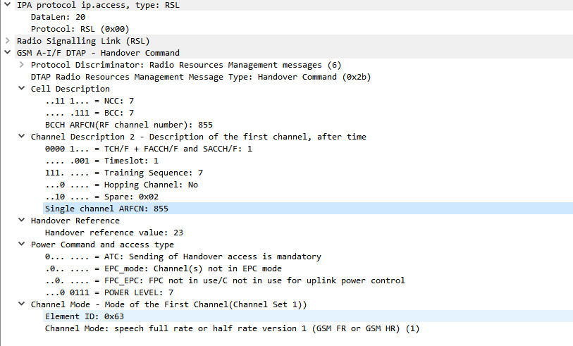
Next a handover command is sent to the phone via the BTS it was initially connected to (RSL Handover Command), telling the phone to begin handover to the new BTS and the channel it should move to on the new BTS it setup earier.
Screenshot of a packet capture showing a GSM Handover
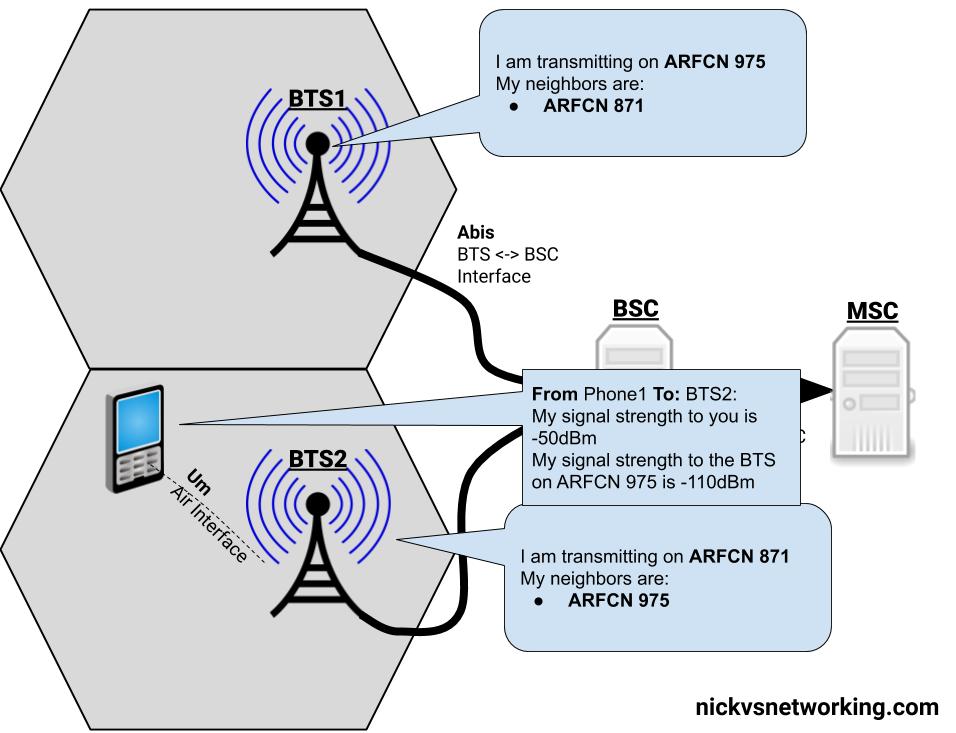
The phone moves to the new BTS, and is acknowledged by the phone. The channels the phone was using on the old BTS are released and the handover is complete.
Simplified Diagram of the Process
There is a lot more to handovers than just this, which we’ll cover in a future post.
This is part of a series of posts focusing on common Diameter request pairs, looking at what’s inside and what they do.
The Authentication Information Request (AIR) and Authentication Information Answer (AIA) are one of the first steps in authenticating a subscriber, and a very common Diameter transaction.
The Process
The Authentication Information Request (AIR) is sent by the MME to the HSS to request when a Subscriber begins to attach containing the IMSI of the subscriber trying to connect.
If the subscriber’s IMSI is known to the HSS, the AuC will generate Authentication Vectors for the Subscriber, and repond back to the MME in an Authentication Information Answer (AIA).
The AIR is a comparatively simple request, without many AVPs;
The Session-Id, Auth-Session-State, Origin-Host, Origin-Realm & Destination-Realm are all common AVPs that have to be included.
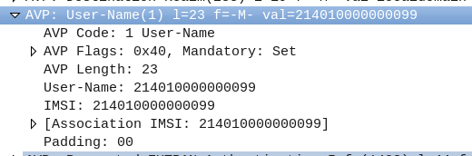
The Username AVP (AVP 1) contains the username of the subscriber, which in this case is the IMSI.
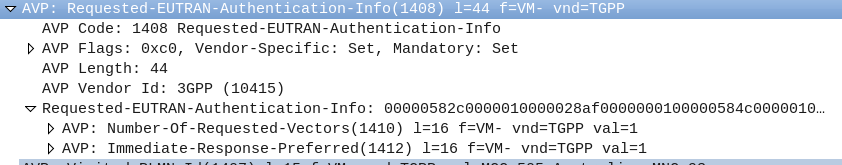
The Requested-EUTRAN-Authentication-Info AVP ( AVP 1408 ) contains information in regards to what authentication info the MME is requesting from the subscriber, typically this indicates the MME is requesting 1 vector (Number-Of-Requested-Vectors (AVP 1410)), an immediate response is preferred (Immediate-Response-Preferred (AVP 1412)), and if the subscriber is re-resyncing the SQN will include a Re-Synchronization-Info AVP (AVP 1411).
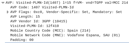
The Visited-PLMN-Id AVP (AVP 1407) contains information regarding the PLMN of the RAN the Subscriber is connecting to.
The Authentication Information Answer (AIA)
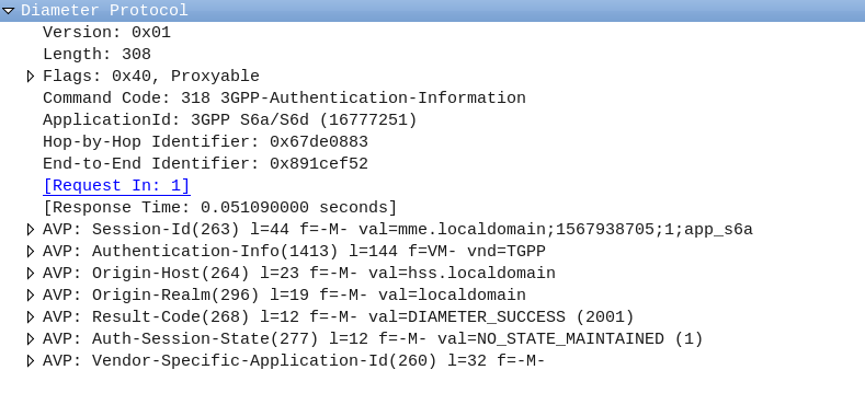
The Authentication Information Answer contains several mandatory AVPs that would be expected, The Session-Id, Auth-Session-State, Origin-Host and Origin-Realm.
The Result Code (AVP 268) indicates if the request was successful or not, 2001 indicates DIAMETER SUCCESS.
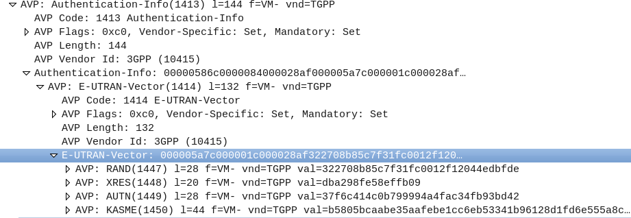
The Authentication-Info (AVP 1413) contains the returned vectors, in LTE typically only one vector is returned, a sub AVP called E-UTRAN-Vector (AVP 1414), which contains AVPs with the RAND, XRES, AUTN and KASME keys.
When setting up the timeslots on the TRX for each BTS on your BSC, you’ll notice you have to set a channel type.
So what do these acronyms mean, and how do they affect the performance of the network?
GSM channels break down into one of to categories, control channels – used for signalling, and traffic channels, used for carrying information to/from a user.
A network with only control channels wouldn’t allow a call to be made, as there would be no traffic channels to carry the audio of the call,
Conversely a network with only traffic channels would have plenty of capacity for calls, but without a control channel would have no way of setting them up.
Traffic Channels
Traffic channels break down into a further two categories, voice channels for carrying call audio, and data channels for carrying GPRS data.
Traffic Channels for Voice
There’s a few variants of voice channel based on the codec used for encoding the voice data, the more compressed / small the audio signal is, the more you can cram in per channel, at the sacrifice of voice quality.
Common options are Traffic Channel – Full Rate (TCH/F), & Traffic Channel – Half Rate (TCH/F) channels.
Traffic Channels for Data
When GPRS was introduced it needed to be transported on a traffic channel, but unlike a voice channel, the resources weren’t going to be used 100% of the time (like in a voice call) and could be shared on an as-needed basis.
Data channels are also also broken down into full rate and half rate channels, like Traffic Channel – Full Rate (TCH/F), & Traffic Channel – Half Rate (TCH/F) channels.
Control Channels
Control channels carry the out of band signalling between the Phone and the BTS.
Broadcast Channels
Broadcast Channels are by their very nature – Broadcasted, this means every phone on the BTS gets these messages.
There are 3 broadcast channels, the FCCH for frequency corrections, SCH for synchronisation and BCCH for a common channel that transmits information to all phones, containing info on the network such as the PLMN, neighbouring cells, etc.
Common Channels
The PCH – Paging Channel, is used to page phones in idle mode. All phones will listen on the paging channel, and if they hear their identifier will establish a connection back to the network.
RACH the Random Access Control Channel is used for when the phone wants to establish a connection with the network, by picking a random timeslot to transmit it’s data on the RACH.
The ACGC is the Access Grant Channel, containing information about dedicated channels to be assigned to phones.
Dedicated Control Channels
Like dedicated traffic channels, dedicated channels are only in use by one phone at a time.
The SDCCH is the standalone dedicated control channel, over which location updates, SMS, authentication & call setup / teardown signalling is transferred.
The SACCH – slow Associated Control Channel is used for timing advance (when users are further from the BTS timing advances are needed to ensure propogation time is taken into account), power control information, signaling data and radio measurements.
Finally the FACCH – Fast Associated Control is used for transferring larger messages such as for handover information,
I’ve written a playbook that provisions some server infrastructure, however one of the steps is to change the hostname.
A common headache when changing the hostname on a Linux machine is that if the hostname you set for the machine, isn’t in the machine’s /etc/hosts file, then when you run sudo su or su, it takes a really long time before it shows you the prompt as the machine struggles to do a DNS lookup for it’s own hostname and fails,
This becomes an even bigger problem when you’re using Ansible to setup these machines, Ansible times out when changing the hostname;
Simple fix, edit the /etc/ansible/ansible.cfg file and include
Depending on if you’re wearing a tin foil hat or not, silent SMS and silent calls could be a useful tool to for administering the network or a backdoor put in to track citizenry!
Regardless of it’s reasons for existence, let’s take a look at what it actually does, and how we can use it.
To conserve battery and radio resources, terminals / UEs go into an idle state where they monitor the RSSI of the BTS/NodeB and the broadcast/paging channels, but don’t actively send anything on the uplink.
Let’s say we wanted to get the RSSI measurements from a terminal/UE we would need the terminal to go into an active state.
We could do this by calling the terminal, or sending an SMS, but if we wanted to do it without alerting the user, that’s when we can use Silent SMS and silent calls, to do so without alerting the user.
If you want to try this you can send a Silent SMS from Osmo-MSC.
Packet capture shows no traffic on the Abis interface until the Silent SMS is sent
On top of Silent SMS there’s also silent calls, allowing for a continued stream of measurements from the UE, which can also be super useful for creating a single call leg.
Another use for Silent SMS it to interface with the SIM Card, many card manufacturers provide support for “over the air” updating of the SIM Card parameters (think if MNO A purchases MNO B and they want to share a network, you don’t want to have to re-issue every SIM card with the updated PLMN, just update the parameters on the SIM).
Messages from the network operator to their SIM cards don’t need to be shown to the user, so are can be carried via Silent SMS. – SIM card manufacturers don’t make the nitty gritty details of this functionality public – it’s a proprietary interface defined by the manufacturer, simply transported by SMS.
In the S1-SETUP-RESPONSE and MME-CONFIGURATION-UPDATE there’s a RelativeMMECapacity (87) IE,
So what does it do?
Most eNBs support connections to multiple MMEs, for redundancy and scalability.
By returning a value from 0 to 255 the MME is able to indicate it’s available capacity to the eNB.
The eNB uses this information to determine which MME to dispatch to, for example:
MME Pool
Relative Capacity
mme001.example.com
20/255
mme002.example.com
230/255
Example MME Pooling table
The eNB with the table above would likely dispatch any incoming traffic to MME002 as MME001 has very little at capacity.
If the capacity was at 1/255 then the MME would very rarely be used.
The exact mechanism for how the MME sets it’s relative capacity is up to the MME implementer, and may vary from MME to MME, but many MMEs support setting a base capacity (for example a less powerful MME you may want to set the relative capacity to make it look more utilised).
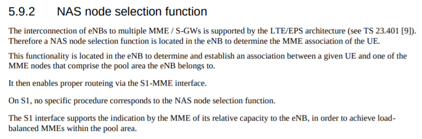
I looked to 3GPP to find what the spec says:
On S1, no specific procedure corresponds to the NAS node selection function. The S1 interface supports the indication by the MME of its relative capacity to the eNB, in order to achieve loadbalanced MMEs within the pool area.
3GPP TS 36.410 – 5.9.2 NAS node selection function