One of the key advantages of SCTP over TCP is the support for Multihoming,
From an application perspective, this enables one “socket”, to be shared across multiple IP Addresses, allowing multiple IP paths and physical NICs.
Through multihoming we can protect against failures in IP Routing and physical links, from a transport layer protocol.
So let’s take a look at how this actually works,
For starters there’s a few ways multihoming can be implemented, ideally we have multiple IPs on both ends (“client” and “server”), but this isn’t always achievable, so SCTP supports partial multi-homing, where for example the client has only one IP but can contact the server on multiple IP Addresses, and visa-versa.
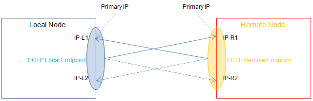
The below image (Courtesy of Wikimedia) shows the ideal scenario, where both the client and the server have multiple IPs they can be reached on.
This would mean a failure of any one of the IP Addresses or the routing between them, would see the other secondary IP Addresses used for Transport, and the application not even necessarily aware of the interruption to the primary IP Path.
The Process
For starters, our SCTP Client/Server will each need to be aware of the IPs that can be used,
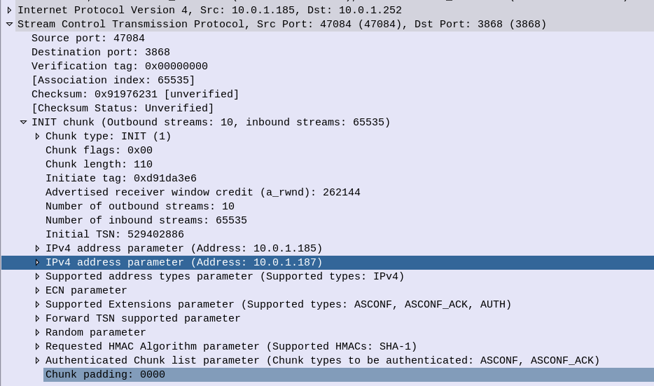
This is advertised in the INIT message, sent by the “client” to a “server” when the SCTP session is established.
SCTP INIT sent by the client at 10.0.1.185, but advertising two IPs
In the above screenshot we can see the two IPs for SCTP to use, the primary IP is the first one (10.0.1.185) and also the from IP, and there is just one additional IP (10.0.1.187) although there could be more.
In a production environment you’d want to ensure each of your IPs is in a different subnet, with different paths, hardware and routes.
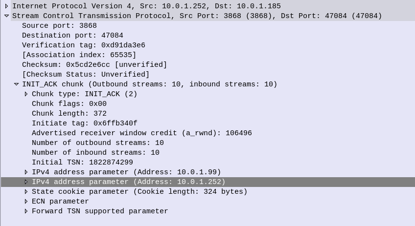
So the INIT is then responded to by the client with an INIT_ACK, and this time the server advertises it’s IP addresses, the primary IP is the From IP address (10.0.1.252) and there is just one additional IP of 10.0.1.99,
SCTP INIT ACK showing Server’s Multi-homed IP Options
Next up we have the cookie exchange, which is used to protect against synchronization attacks, and then our SCTP session is up.
So what happens at this point? How do we know if a path is up and working?
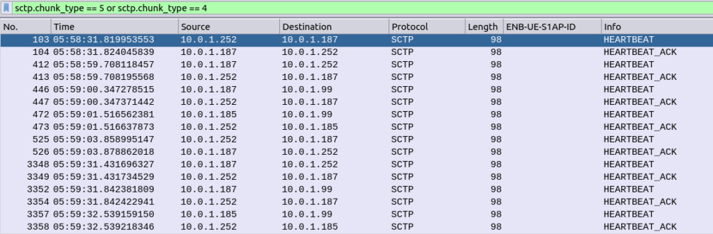
Well the answer is heartbeat messages,
Sent from each of the IPs on the client to each of the IPs on the server, to make sure that there’s a path from every IP, to every other IP.
SCTP Heartbeats from each local IP to each remote IP
This means the SCTP stacks knows if a path fails, for example if the route to IP 10.0.1.252 on the server were to fail, the SCTP stack knows it has another option, 10.0.1.99, which it’s been monitoring.
So that’s multi-homed SCTP in action – While a lot of work has historically been done with LACP for aggregating multiple NICs together, and VRRP for ensuring a host is alive, SCTP handles this in a clean and efficient way.
I’ve attached a PCAP showing multi-homing on a Diameter S6a (HSS) interface between an MME and a HSS.
So dedicated appliances are dead and all our network functions are VMs or Containers, but there’s a performance hit when going virtual as the L2 processing has to be handled by the Hypervisor before being passed onto the relevant VM / Container.
If we have a 10Gb NIC in our server, we want to achieve a 10Gbps “Line Speed” on the Network Element / VNF we’re running on.
When we talked about appliances if you purchased an P-GW with 10Gbps NIC, it was a given you could get 10Gbps through it (without DPI, etc), but when we talk about virtualized network functions / network elements there’s a very real chance you won’t achieve the “line speed” of your interfaces without some help.
When you’ve got a Network Element like a S-GW, P-GW or UPF, you want to forward packets as quickly as possible – bottlenecks here would impact the user’s achievable speeds on the network.
To speed things up there are two technologies, that if supported by your software stack and hardware, allows you to significantly increase throughput on network interfaces, DPDK & SR-IOV.
DPDK – Data Plane Development Kit
Usually *Nix OSs handle packet processing on the Kernel level. As I type this the packets being sent to this WordPress server by Firefox are being handled by the Linux 5.8.0-36-generic kernel running on my machine.
The problem is the kernel has other things to do (interrupts), meaning increased delay in processing (due to waiting for processing capability) and decreased capacity.
DPDK shunts this processing to the “user space” meaning your application (the actual magic of the VNF / Network Element) controls it.
To go back to me writing this – If Firefox and my laptop supported DPDK, then the packets wouldn’t traverse the Linux kernel at all, and Firefox would be talking directly to my NIC. (Obviously this isn’t the case…)
So DPDK increases network performance by shifting the processing of packets to the application, bypassing the kernel altogether. You are still limited by the CPU and Memory available, but with enough of each you should reach very near to line speed.
SR-IOV – Single Root Input Output Virtualization
Going back to the me writing this analogy I’m running Linux on my laptop, but let’s imagine I’m running a VM running Firefox under Linux to write this.
If that’s the case then we have an even more convolted packet processing chain!
I type the post into Firefox which sends the packets to the Linux kernel, which waits to be scheduled resources by the hypervisor, which then process the packets in the hypervisor kernel before finally making it onto the NIC.
We could add DPDK which skips some of these steps, but we’d still have the bottleneck of the hypervisor.
With PCIe passthrough we could pass the NIC directly to the VM running the Firefox browser window I’m typing this, but then we have a problem, no other VMs can access these resources.
SR-IOV provides an interface to passthrough PCIe to VMs by slicing the PCIe interface up and then passing it through.
My VM would be able to access the PCIe side of the NIC, but so would other VMs.
So that’s the short of it, SR-IOR and DPDK enable better packet forwarding speeds on VNFs.
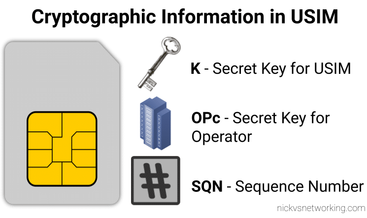
While we’ve already covered the inputs required by the authentication elements of the core network (The HSS in LTE/4G, the AuC in UMTS/3G and the AUSF in 5G) to generate an output, it’s worth noting that the Confidentiality Algorithms used in the process determines the output.
This means the Authentication Vector (Also known as an F1 and F1*) generated for a subscriber using Milenage Confidentiality Algorithms will generate a different output to that of Confidentiality Algorithms XOR or Comp128.
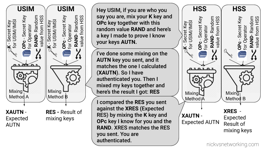
To put it another way – given the same input of K key, OPc Key (or OP key), SQN & RAND (Random) a run with Milenage (F1 and F1* algorithm) would yield totally different result (AUTN & XRES) to the same inputs run with a simple XOR.
Technically, as operators control the network element that generates the challenges, and the USIM that responds to them, it is an option for an operator to implement their own Confidentiality Algorithms (Beyond just Milenage or XOR) so long as it produced the same number of outputs. But rolling your own cryptographic anything is almost always a terrible idea.
So what are the differences between the Confidentiality Algorithms and which one to use? Spoiler alert, the answer is Milenage.
Milenage
Milenage is based on AES (Originally called Rijndael) and is (compared to a lot of other crypto implimentations) fairly easy to understand,
AES is very well studied and understood and unlike Comp128 variants, is open for anyone to study/analyse/break, although AES is not without shortcomings, it’s problems are at this stage, fairly well understood and mitigated.
There are a few clean open source examples of Milenage implementations, such as this C example from FreeBSD.
XOR
It took me a while to find the specifications for the XOR algorithm – it turns out XOR is available as an alternate to Milenage available on some SIM cards for testing only, and the mechanism for XOR Confidentiality Algorithm is only employed in testing scenarios, not designed for production.
Instead of using AES under the hood like Milenage, it’s just plan old XOR of the keys.
Comp128 was originally a closed source algorithm, with the maths behind it not publicly available to scrutinise. It is used in GSM A3 and A5 functions, akin to the F1 and F1* in later releases.
Due to its secretive nature it wasn’t able to be studied or analysed prior to deployment, with the idea that if you never said how your crypto worked no one would be able to break it. Spoiler alert; public weaknesses became exposed as far back as 1998, which led to Toll Fraud, SIM cloning and eventually the development of two additional variants, with the original Comp128 renamed Comp128-1, and Comp128-2 (stronger algorithm than the original addressing a few of its flaws) and Comp128-3 (Same as Comp128-2 but with a 64 bit long key generated).
Instead of going to all the effort of creating VMs (or running Ansible playbooks) we can use Docker and docker-compose to create a test environment with multiple Asterisk instances to dispatch traffic to from Kamailio.
I covered the basics of using Kamailio with Docker in this post, which runs a single Kamailio instance inside Docker with a provided config file, but in this post we’ll use docker-compose to run multiple Asterisk instances and setup Kamailio to dispatch traffic to them.
I am a big Kubernetes fan, and yes, all this can be done in Kubernetes, and would be a better fit for a production environment, but for a development environment it’s probably overkill.
#Copy the config file onto the Filesystem of the Docker instance
COPY dispatcher.list /etc/kamailio/
COPY kamailio.cfg /etc/kamailio/
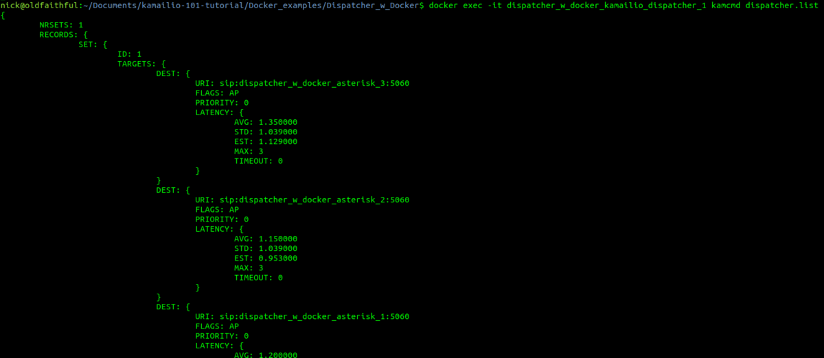
The Kamailio config we’re using is very similar to the Dispatcher example but with a few minor changes to the timers and setting it to use the Dispatcher data from a text file instead of a database. If you have a look at the contents of dispatcher.list you’ll see three entries; dispatcher_w_docker_asterisk_1, dispatcher_w_docker_asterisk_2 & dispatcher_w_docker_asterisk_3. These will be the hostnames of the 3 Asterisk instances we’ll create.
Next up we’ll take a look at the docker-compose file, which defines how our environment will be composed, and defines which containers will be run
The docker-compose file contains definitions about the Containers we want to run, for this example we’ll run several Asterisk instances and a single Kamailio instance.
The replicas: 6 parameter is ignored by standard docker-compose up command, but will be used if you’re using Docker swarm, otherwise we’ll manually set the number of replicas when we run the command.
So with that defined let’s define our Kamailio service;
So far with most of our discussions about Kamailio we’ve talked about routing the initial SIP request (INVITE, REGISTER, SUBSCRIBE, etc), but SIP is not a one-message protocol, there’s a whole series of SIP messages that go into a SIP Dialog.
Sure the call may start with an INVITE, but there’s the 180 RINGING, the 200 OK and the ACK that go into getting the call actually established, and routing these in-dialog messages is just as important as routing the first INVITE.
When we’ve talked about SIP routing it’s all happened in the request_route {} block:
request_route {
        xlog("Received $rm to $ru - Forwarding");
        append_hf("X-Proxied: You betcha\r\n");
        #Forward to new IP
        forward("192.168.1.110");
}
In the example above we statelessly forward any initial requests to the IP 192.168.1.110.
We can add an onreply_route{} block to handle any replies from 192.168.1.110 back to the originator.
But why would we want to?
Some simple answers would be to do some kind of manipulation to the message – say to strip a Caller ID if CLIP is turned off, or to add a custom SIP header containing important information, etc.
onreply_route{
        xlog("Got a reply $rs");
        append_hf("X-Proxied: For the reply\r\n");
}
Let’s imagine a scenario where the destination our SIP proxy is relaying traffic to (192.168.1.110) starts responding with 404 error.
We could detect this in our onreply_route{} and do something about it.
onreply_route{
        xlog("Got a reply $rs");
        if($rs == 404) {
                #If remote destination returns 404
                xlog("Got a 404 for $rU");
                #Do something about it
        }
}
In the 404 example if we were using Dispatcher it’s got easily accessed logic to handle these scenarios a bit better than us writing it out here, but you get the idea.
There are a few other special routes like onreply_route{}, failure routes and event routes, etc.
Hopefully now you’ll have a better idea of how and when to use onreply_route{} in Kamailio.
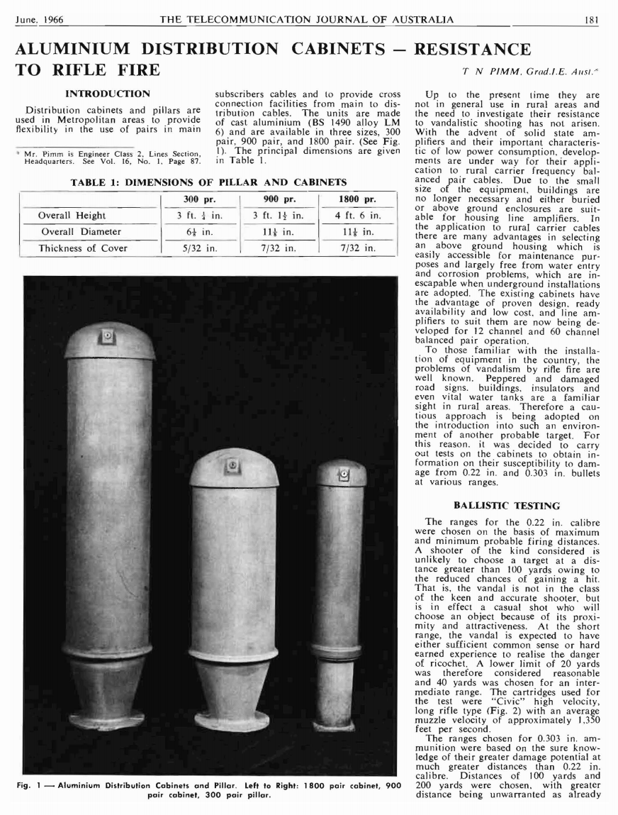
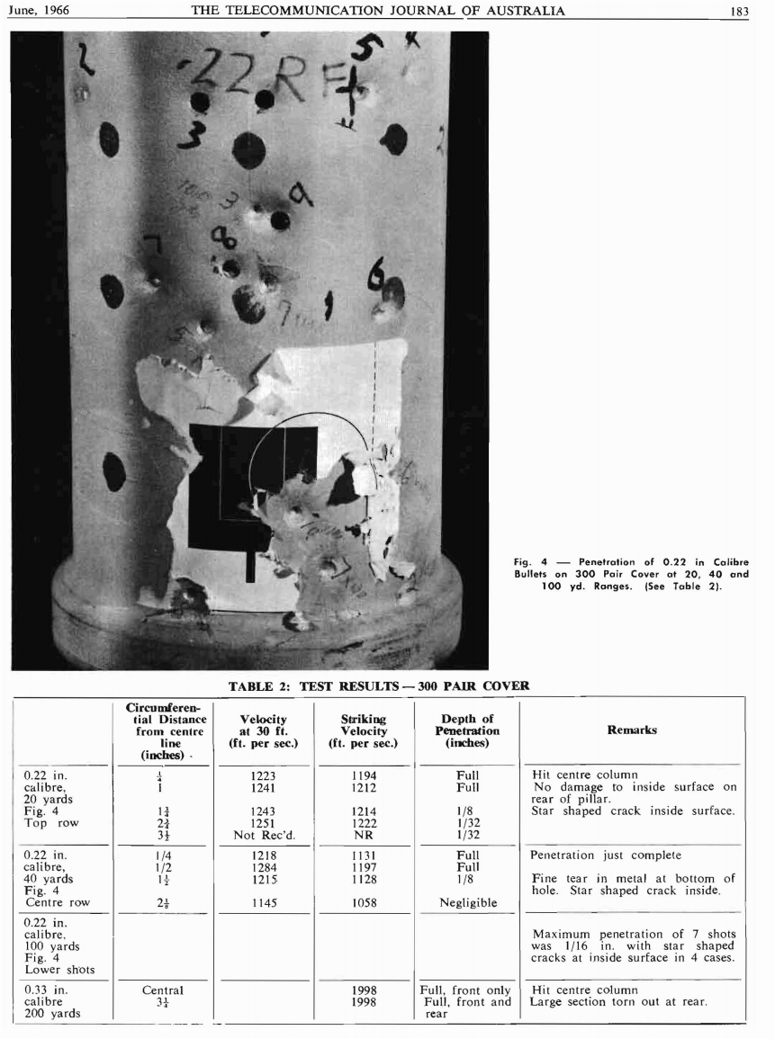
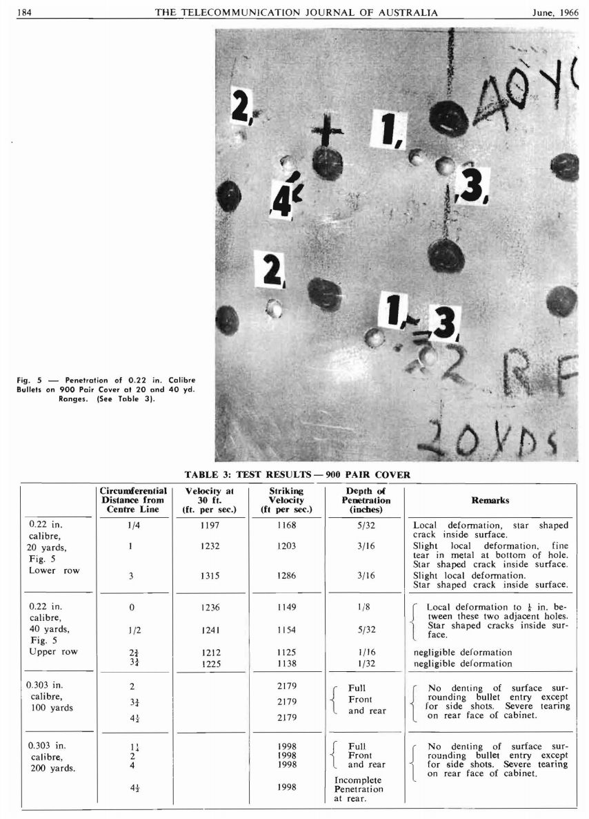
The 900 and 1800 pair telecom distribution pillars (aka cabinets) are still a familiar sight almost everywhere in Australia where copper networks are still used, however prior to the early 1970s they were only deployed in metropolitan areas, and apparently one of the concerns of deploying them in rural areas was that they’d be shot at.
June 1966 issue of the Telecommunications Journal of Australia (TJA) has an article titled “Aluminum Distribution Cabinets – Resistance to Rifle Fire” is below, click to get the image full size.
At the short range, the vandal is expected to have either sufficient common sense or hard earned experience to realise the danger of ricochet.
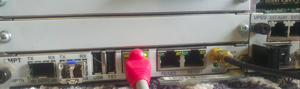
Our BTS is going to need an accurate clock source in order to run, so without access to crazy accurate Timing over Packet systems or TDM links to use as reference sources, I’ve opted to use the GPS/GLONASS receiver built into the LMPT card.
Add new GPS with ID 0 on LMPT in slot 7 of cabinet 1:
Check GPS has sync (May take some time) using the Display GPS command;
DSP GPS: GN=0;
Assuming you’ve got an antenna connected and can see the sky, after ~10 minutes running the DSP GPS:; command again should show you an output like this:
+++    4-PAL0089624        2020-11-28 01:06:55
O&M    #806355684
%%DSP GPS: GN=0;%%
RETCODE = 0  Operation succeeded.

Display GPS State
-----------------
                 GPS Clock No.  =  0
                GPS Card State  =  Normal
                 GPS Card Type  =  M12M
                 GPS Work Mode  =  GPS
                   Hold Status  =  UNHOLDED
         GPS Satellites Traced  =  4
     GLONASS Satellites Traced  =  0
         BDS Satellites Traced  =  0
Antenna Longitude(1e-6 degree)  =  144599999
 Antenna Latitude(1e-6 degree)  =  -37000000
           Antenna Altitude(m)  =  613
         Antenna Angle(degree)  =  5
             Link Active State  =  Activated
              Feeder Delay(ns)  =  15
                   GPS Version  =  NULL
(Number of results = 1)


---    END
Showing the GPS has got sync and a location fix,
Next we set BTS to use GPS as time source,
SET TIMESRC: TIMESRC=GPS;
Finally we’ll verify the Time is in sync on the BTS using the list time command:
DSP TIME:;
+++    4-PAL0089624        2020-11-28 01:09:22
O&M    #806355690
%%DSP TIME:;%%
RETCODE = 0  Operation succeeded.

Time Information
----------------
Time  =  2020-11-28 01:09:22 GMT+00:00

---    END
Optionally you may wish to add a timezone, using the SET TZ:; command, but I’ve opted to keep it in UTC for simplicity.
In our last post we covered the file system structure of a smart card and the basic concepts of communication with cards. In this post we’ll look at what happens on the application layer, and how to interact with a card.
For these examples I’ll be using SIM cards, because admit it, you’ve already got a pile sitting in a draw, and this is a telco blog after all. You won’t need the ADM keys for the cards, we’ll modify files we’ve got write access to by default.
Commands & Instructions
So to do anything useful with the card we need issue commands / instructions to the card, to tell it to do things. Instructions like select this file, read it’s contents, update the contents to something else, verify my PIN, authenticate to the network, etc.
The term Command and Instruction are used somewhat interchangeably in the spec, I realise that I’ve done the same here to make it just as confusing, but instruction means the name of the specific command to be called, and command typically means the APDU as a whole.
The “Generic Commands” section of 3GPP TS 31.101 specifies the common commands, so let’s take a look at one.
The creatively named SELECT command/instruction is used to select the file we want to work with. In the SELECT command we’ll include some parameters, like where to find the file, so some parameters are passed with the SELECT Instruction to limit the file selection to a specific area, etc, the length of the file identifier to come, and the identifier of the file.
The card responds with a Status Word, returned by the card, to indicate if it was successful. For example if we selected a file that existed and we had permission to select, we’d get back a status word indicating the card had successfully selected the file. Status Words are 2 byte responses that indicate if the instruction was successful, but also the card has data it wants to send to the terminal as a result of the instruction, how much data the terminal should expect.
So if we just run a SELECT command, telling the card to select a file, we’ll get back a successful response from the card with a data length. Next need to get that data from the card. As the card can’t initiate communication, the GET RESPONSE instruction is sent to the card to get the data from the card, along with the length of the data to be returned.
The GET RESPONSE instruction/command is answered by the card with an APDU containing the data the card has to send, and the last 2 bytes contain the Status Word indicating if it was successful or not.
APDUs
So having covered the physical and link layers, we now move onto the Application Layer – where the magic happens.
Smart card communications is strictly master-slave based when it comes to the application layer.
The terminal sends a command to the card, which in turn sends back a response. Command -> Response, Command -> Response, over and over.
These commands are contained inside APplication Data Units (APDUs).
So let’s break down a simple APDU as it appears on the wire, so to speak.
The first byte of our command APDU is taken up with a header called the class byte, abbreviated to CLA. This specifies class coding, secure messaging options and channel options.
In the next byte we specify the Instruction for the command, that’s the task / operation we want the card to perform, in the spec this is abbreviated to INS.
The next two bytes, called P1 & P2 (Parameter 1 & Parameter 2) specify the parameters of how the instruction is to be to be used.
Next comes Lc – Length of Command, which specifies the length of the command data to follow,
Datacomes next, this is instruction data of the length specified in Lc.
Finally an optional Le – Length of expected response can be added to specify how long the response from the card should be.
Crafting APDUs
So let’s encode our own APDU to send to a card, for this example we’ll create the APDU to tell the card to select the Master File (MF) – akin to moving to the root directory on a *nix OS.
For this we’ll want a copy of ETSI TS 102 221 – the catchily named “Smart cards; UICC-Terminal interface; Physical and logical characteristics” which will guide in the specifics of how to format the command, because all the commands are encoded in hexadecimal format.
So here’s the coding for a SELECT command from section 11.1.1.1 “SELECT“,
For the CLA byte in our example we’ll indicate in our header that we’re using ISO 7816-4 encoding, with nothing fancy, which is denoted by the byte A0.
For the next but we’ve got INS (Instruction) which needs to be set to the hex value for SELECT, which is represented by the hex value A4, so our second byte will have that as it’s value.
The next byte is P1, which specifies “Selection Control”, the table in the specification outlines all the possible options, but we’ll use 00 as our value, meaning we’ll “Select DF, EF or MF by file id”.
The next byte P2 specifies more selection options, we’ll use “First or only occurrence” which is represented by 00.
The Lc byte defines the length of the data (file id) we’re going to give in the subsequent bytes, we’ve got a two byte File ID so we’ll specify 2 (represented by 02).
Finally we have the Data field, where we specify the file ID we want to select, for the example we’ll select the Master File (MF) which has the file ID ‘3F00‘, so that’s the hex value we’ll use.
So let’s break this down;
Code
Meaning
Value
CLA
Class bytes – Coding options
A0 (ISO 7816-4 coding)
INS
Instruction (Command) to be called
A4 (SELECT)
P1
Parameter 1 – Selection Control (Limit search options)
00 (Select by File ID)
P2
Parameter 1 – More selection options
00 (First occurrence)
Lc
Length of Data
02 (2 bytes of data to come)
Data
File ID of the file to Select
3F00 (File ID of master file)
So that’s our APDU encoded, it’s final value will be A0 A4 00 00 02 3F00
So there we have it, a valid APDU to select the Master File.
In the next post we’ll put all this theory into practice and start interacting with a real life SIM cards using PySIM, and take a look at the APDUs with Wireshark.
The pins on the terminal / card reader are arranged so that when inserting a card, the ground contact is the first contact made with the reader, this clever design consideration to protect the card and the reader from ESD damage.
Operating Voltages
When Smart Cards were selected for use in GSM for authenticating subscribers, all smart cards operated at 5v. However as mobile phones got smaller, the operating voltage range became more limited, the amount of space inside the handset became a premium and power efficiency became imperative. The 5v supply for the SIM became a difficult voltage to provide (needing to be buck-boosted) so lower 3v operation of the cards became a requirement, these cards are referred to as “Class B” cards. This has since been pushed even further to 1.8v for “Class C” cards.
If you found a SIM from 1990 it’s not going to operate in a 1.8v phone, but it’s not going to damage the phone or the card.
The same luckily goes in reverse, a card designed for 1.8v put into a phone from 1990 will work just fine at 5v.
This is thanks to the class flag in the ATR response, which we’ll cover later on.
Clocks
As we’re sharing one I/O pin for TX and RX, clocking is important for synchronising the card and the reader. But when smart cards were initially designed the clock pin on the card also served as the clock for the micro controller it contained, as stable oscillators weren’t available in such a tiny form factor. Modern cards implement their own clock, but the clock pin is still required for synchronising the communication.
I/O Pin
The I/O pin is used for TX & RX between the terminal/phone/card reader and the Smart Card / SIM card. Having only one pin means the communications is half duplex – with the Terminal then the card taking it in turns to transmit.
Reset Pin
Resets the card’s communications with the terminal.
Filesystem
So a single smart card can run multiple applications, the “SIM” is just an application, as is USIM, ISIM and any other applications on the card.
These applications are arranged on a quasi-filesystem, with 3 types of files which can be created, read updated or deleted. (If authorised by the card.)
Because the file system is very basic, and somewhat handled like a block of contiguous storage, you often can’t expand a file – when it is created the required number of bytes are allocated to it, and no more can be added, and if you add file A, B and C, and delete file B, the space of file B won’t be available to be used until file C is deleted.
This is why if you cast your mind back to when contacts were stored on your phone’s SIM card, you could only have a finite number of contacts – because that space on the card had been allocated for contacts, and additional space can no longer be allocated for extra contacts.
So let’s take a look at our 3 file types:
MF (Master File)
The MF is like the root directory in Linux, under it contains all the files on the card.
DF (Dedciated File)
An dedicated file (DF) is essentially a folder – they’re sometimes (incorrectly) referred to as Directory Files (which would be a better name).
They contain one or more Elementary Files (see below), and can contain other DFs as well.
Dedicated Files make organising the file system cleaner and easier. DFs group all the relevant EFs together. 3GPP defines a dedicated file for Phonebook entries (DFphonebook), MBMS functions (DFtv) and 5G functions (DF5gs).
We also have ADFs – Application Dedicated Files, for specific applications, for example ADFusim contains all the EFs and DFs for USIM functionality, while ADFgsm contains all the GSM SIM functionality.
The actual difference with an ADF is that it’s not sitting below the MF, but for the level of depth we’re going into it doesn’t matter.
DFs have a name – an Application Identifier (AID) used to address them, meaning we can select them by name.
EF (Elementary File)
Elementary files are what would actually be considered a file in Linux systems.
Like in a Linux file systems EFs can have permissions, some EFs can be read by anyone, others have access control restrictions in place to limit who & what can access the contents of an EF.
There are multiple types of Elementary Files; Linear, Cyclic, Purse, Transparent and SIM files, each with their own treatment by the OS and terminal.
Most of the EFs we’ll deal with will be Transparent, meaning they ##
ATR – Answer to Reset
So before we can go about working with all our files we’ll need a mechanism so the card, and the terminal, can exchange capabilities.
There’s an old saying that the best thing about standards is that there’s so many to choose, from and yes, we’ve got multiple variants/implementations of the smart card standard, and so the card and the terminal need to agree on a standard to use before we can do anything.
This is handled in a process called Answer to Reset (ATR).
When the card is powered up, it sends it’s first suggestion for a standard to communicate over, if the terminal doesn’t want to support that, it just sends a pulse down the reset line, the card resets and comes back with a new offer.
If the card offers a standard to communicate over that the terminal does like, and does support, the terminal will send the first command to the card via the I/O line, this tells the card the protocol preferences of the terminal, and the card responds with it’s protocol preferences. After that communications can start.
Basic Principles of Smart Cards Communications
So with a single I/O line to the card, it kind of goes without saying the communications with the card is half-duplex – The card and the terminal can’t both communicate at the same time.
Instead a master-slave relationship is setup, where the smart card is sent a command and sends back a response. Command messages have a clear ending so the card knows when it can send it’s response and away we go.
Like most protocols, smart card communications is layered.
At layer 1, we have the physical layer, defining the operating voltages, encoding, etc. This is standardised in ISO/IEC 7816-3.
Above that comes our layer 2 – our Link Layer. This is also specified in ISO/IEC 7816-3, and typically operates in one of two modes – T0 or T1, with the difference between the two being one is byte-oriented the other block-oriented. For telco applications T0 is typically used.
Our top layer (layer 7) is the application layer. We’ll cover the details of this in the next post, but it carries application data units to and from the card in the form of commands from the terminal, and responses from the card.
Coming up Next…
In the next post we’ll look into application layer communications with cards, the commands and the responses.