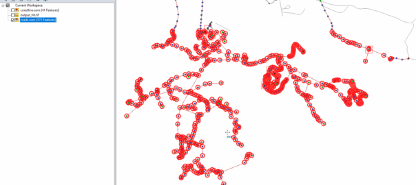
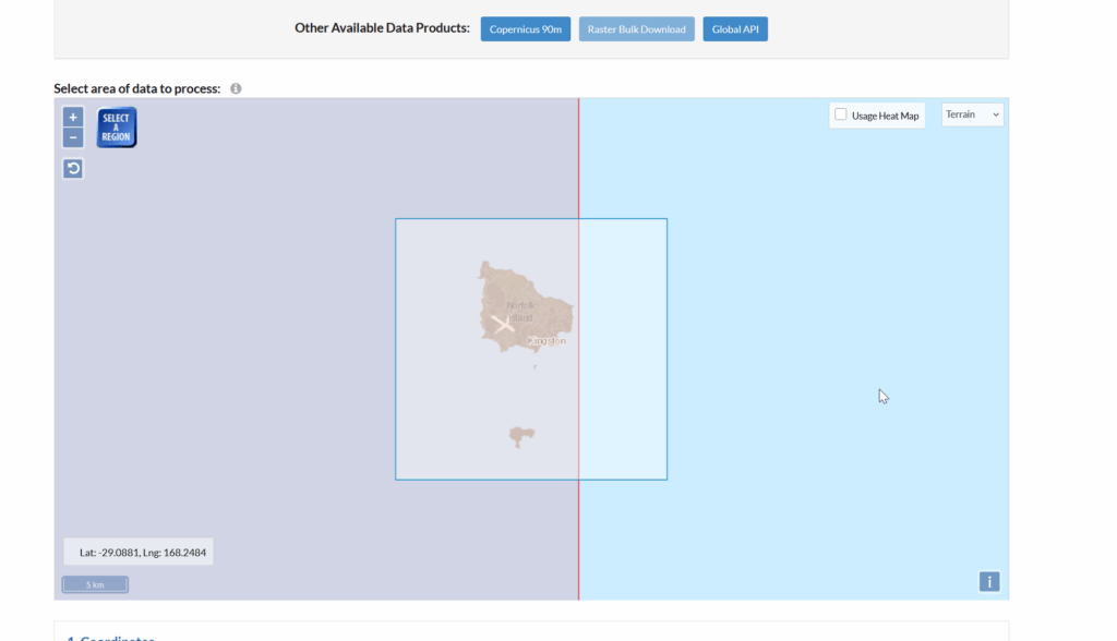
Looks like this is my 3rd (and hopefully final) post on the topic of loading Digital Elevation Models / Topographic data into Forsk Atoll, because this time, we’ve got global data, which allows us to Digital Elevation Models, at 30m resolution, for anywhere on the planet.
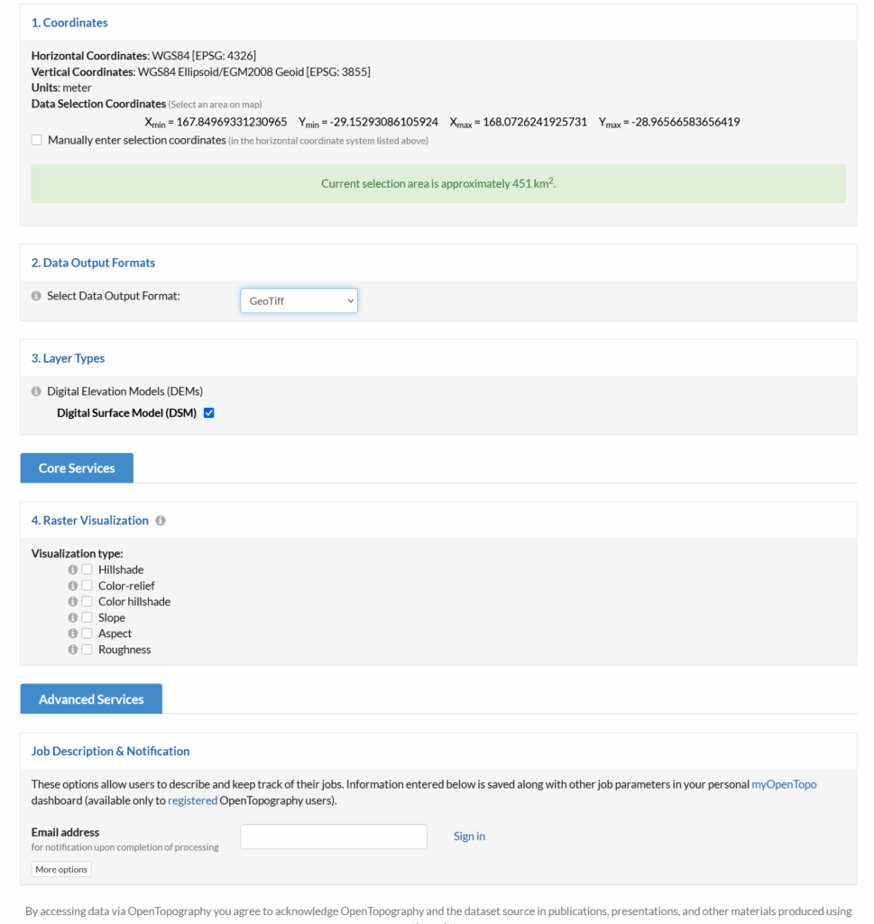
The Copernicus DEM is a Digital Surface Model (DSM) which represents the surface of the Earth including buildings, infrastructure and vegetation. This DSM is derived from an edited DSM named WorldDEM, where flattening of water bodies and consistent flow of rivers has been included. In addition, editing of shore- and coastlines, special features such as airports, and implausible terrain structures has also been applied.
The WorldDEM product is based on the radar satellite data acquired during the TanDEM-X Mission, which is funded by a Public Private Partnership between the German State, represented by the German Aerospace Centre (DLR) and Airbus Defence and Space. OpenTopography is providing access to the global GLO-30 Defence Gridded Elevation Data (DGED) 2023_1 version of the data hosted by ESA via the PRISM service. Details on the Copernicus DSM can be found on this ESA site.
This is a tool for a job, 30m resolution is not crazy high – LIDAR scans achieve sub 1m accuracy, but aren’t available everywhere, where as the COP30 dataset is global, meaning we can do RF design for anywhere on the planet.
So how do we get this into Atoll to do RF modeling?
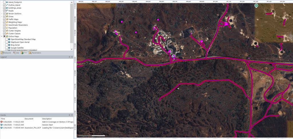
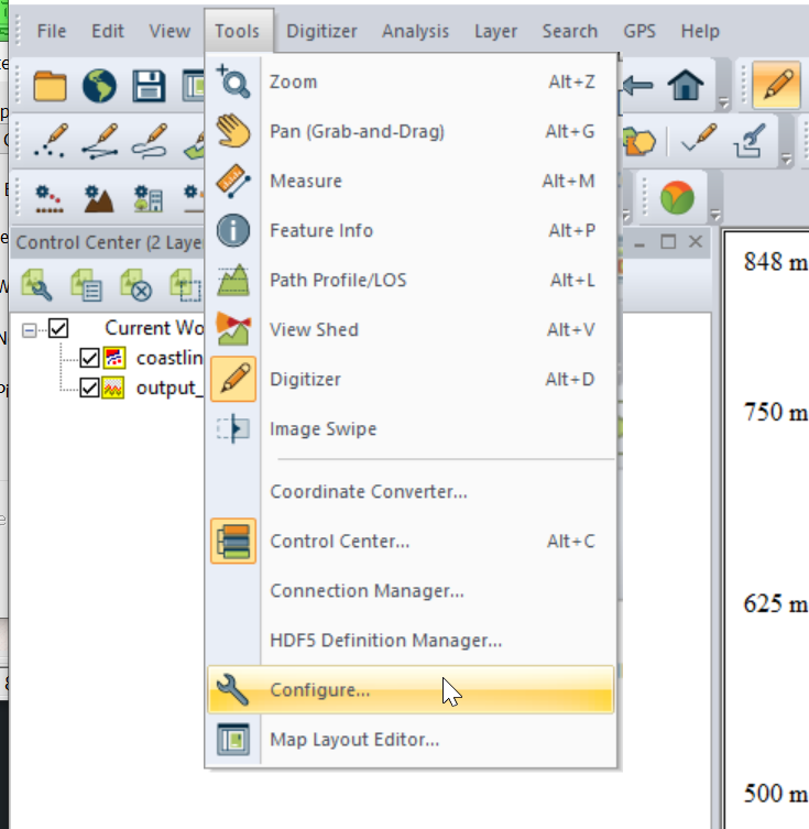
I had to re-project the data, so inside Global Mapper I had to go to Tools -> Configure.
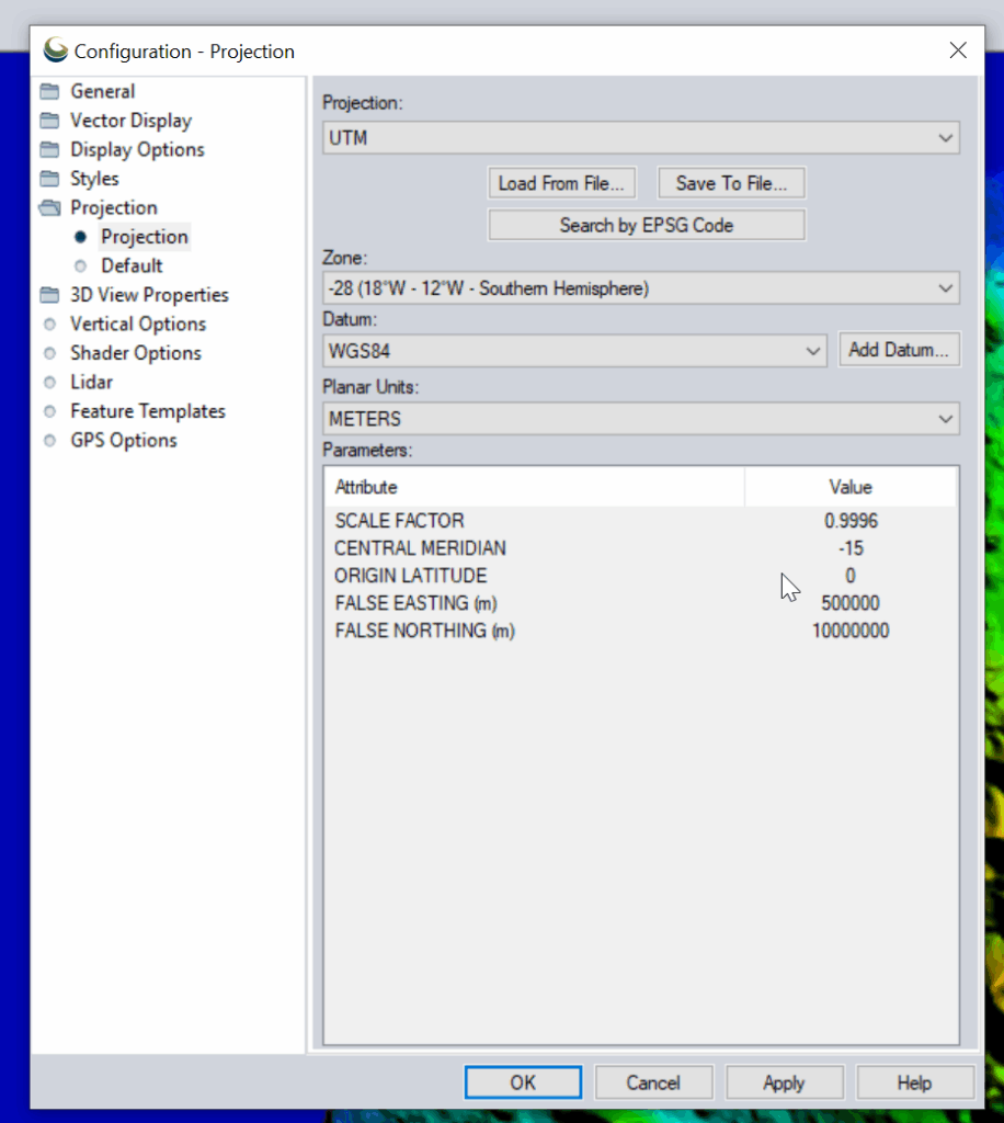
Then change the projection to UTM and use the UTM Zone Finder to find out what zone I needed.
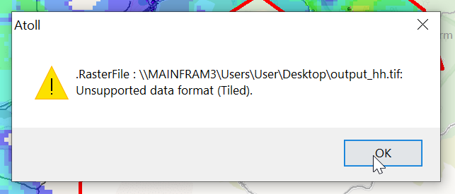
Then I exported the data as an Erdas Imagine file and was able to imported happily into Atoll, after setting the matching projection in Atoll (Which you generally do at the start of the project).
Some questions I wanted to impirically answer with Elixir:
Does the size of value of a Map or ETS object impact the time it takes to retrive a given record (specifically to find that key from others)?
Does the number of keys in ETS or a Map impact the time it takes to retrive a given record?
So what did I find:
Question: Does the size of value of a Map or ETS object impact the time it takes to retrive a given record (specifically to find that key from others)?
Answer: In Maps, the impact of a 100x larger payload being written has a fairly minimal (4% impact) on read speed, but this is ~30% when using ETS.
Methodology used:
Compared 100000 and 100 byte payloads for read and write times.
ETS Write is 24% slower with the larger payload (That’s to be expected, we’ve got more data to copy)
ETS Read is 30% slower with the larger payload (Suggests that the size of the payload has a bearing on how quickly it can be indexed)
Map Write was 13% slower with the larger payload and the Map read is only 4% slower
=== Results === Payload gen: 0 ms for 100000 bytes
ETS write: 223 ms (448,430.5 writes/sec) ETS read: 15933 ms total (933,910.8 reads/sec)
Map write: 108 ms (925,925.9 writes/sec) Map read: 2355 ms total (6,318,471.3 reads/sec)
  @reads 14_880_000
  @distinct 100_000
  @payload_bytes 100
=== Results ===
Payload gen: 0 ms for 100 bytes

ETS write:   177 ms (564,971.8 writes/sec)
ETS read:    11149 ms total (1,334,648.8 reads/sec)

Map write:   125 ms (800,000.0 writes/sec)
Map read:    2470 ms total (6,024,291.5 reads/sec)
Question: Does the number of keys in ETS or a Map impact the time it takes to retrive a given record?
Answer: Writing 1000 records is of course super quick. That much should be obvious, but the retrive / read time is what I’m interested in here.
ETS: Yes, there is a ~40% performance hit in retriving a record from an ETS DB with 14m records than a DB with 1k records. This doesn’t appear to be linear, but there is an impact.
Map: Boy howdy, there’s a 10x increase in the time to get data when the database is larger than smaller. This is probably to do with how simple Maps are, compared to ETS which is definatley a better tool for the job when working with more records.
This led to an interesting realization, Map is faster at smaller sets of data (more keys, not larger values), but ETS is faster for larger data sets (again more keys, not coutning the values), and there’s a break-even point for ETS usage.
TL;DR – ETS – Number of keys has a mangable impact (40%) on retrive time. Map – Number of keys has a very real impact (10x) impact on read times.
Compared 1000 distinct keys vs 14.8m distinct keys.
  @reads 14_880_000
  @distinct 1000
  @payload_bytes 1000
ETS write:   1 ms (1,000,000.0 writes/sec)
ETS read:    9769 ms total (1,523,185.6 reads/sec)

Map write:   9 ms (111,111.1 writes/sec)
Map read:    1292 ms total (11,517,027.9 reads/sec)
  @reads 14_880_000
  @distinct 14_880_000
  @payload_bytes 1000
ETS write:   26176 ms (568,459.7 writes/sec)
ETS read:    16363 ms total (909,368.7 reads/sec)

Map write:   45503 ms (327,011.4 writes/sec)
Map read:    12926 ms total (1,151,168.2 reads/sec)
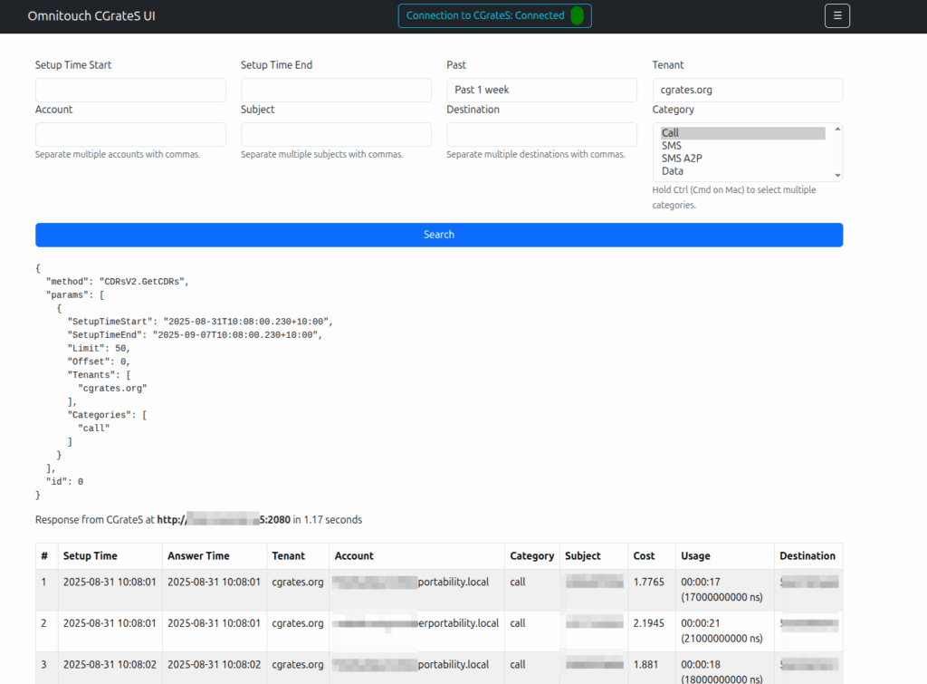
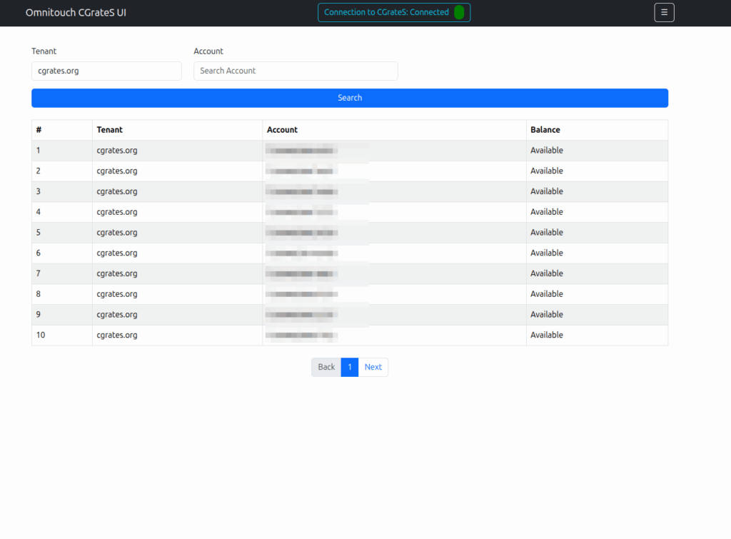
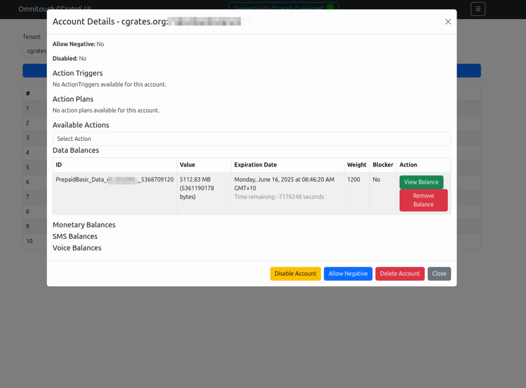
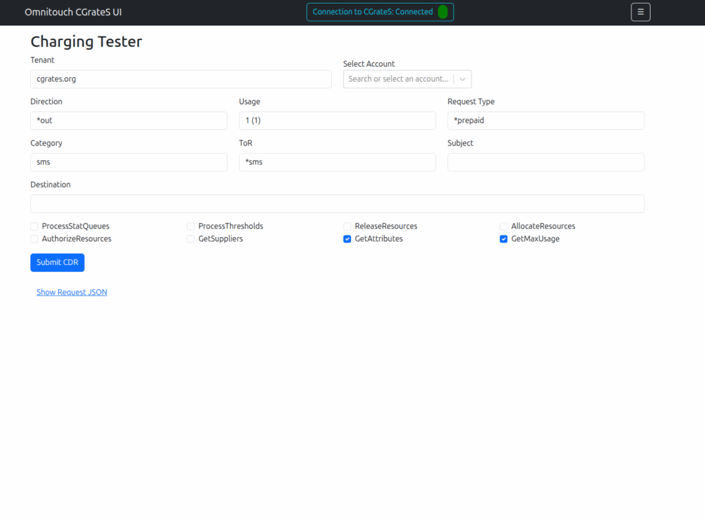
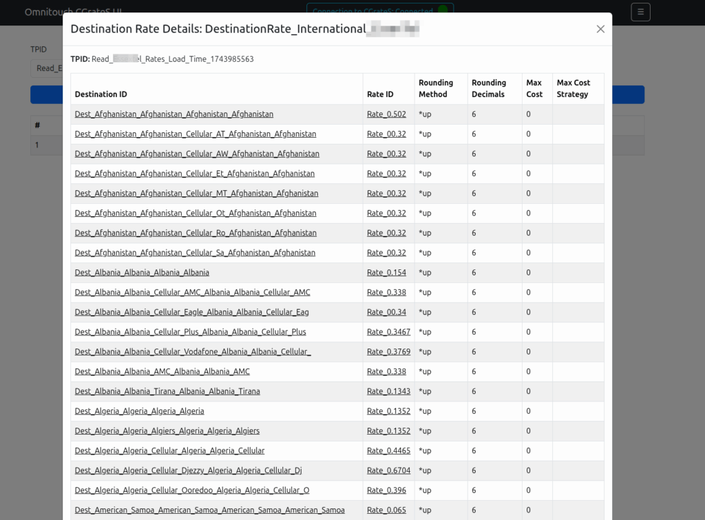
Working a lot with CGrateS I found myself doing the same tasks somewhat regularly, one common task was being asked to get CDRs for a certain thing on an ad-hoc basis, ie “Can you get the call records for XXXX for last month?” or “How much did we spend on calls to YY this quarter?” or “How many GB of data did roamers use on these 3 cell cites this week?”
As those were all CDR related queries, I knocked up a quick React Web UI to search CDRs.
Then we introduced accounts with balances, and there were queries about checking balances, adding roaming packs, etc.
And then things just kinda spiraled…
Managing Actions and Action Plans, rates, simulating cost, Attributes, SessionS, etc, etc.
This isn’t meant as a GUI – If you don’t know how CGrateS works, this tool won’t help you.
But if you’re already working with CGrateS and sending random HTTP POSTs of JSON blobs from your language of choice, this a toolbox to manipulate data will hopefully be useful to you.
I think of it as kinda like Postman but a bit simpler and just focused on CGrateS.
At the time of writing it can view/manage: Searching and exporting CDRs
I’ve been facing an issue in Vscode for a long time where when I’ve printed a lot of data to the terminal, everything gets really unresponsive – Scrolling through the results is like I’m drunk it’s so unresponsive, and I’ve tried a bunch of stuff to fix it.
Here’s the Benchee benchmarks for a function in Elixir that happens to print a lot of data to the terminal, if I run it in Vscode:
A meagre 12.4 IPS on that function, but not only that but I see the CPU usage spike and the computer becomes unsuable.
But if I run in Ubuntu’s default terminal (GNOME Terminal):
5 fold increase and I don’t even see CPU spike above 30%.
So what gives?
Here’s what I’ve tried:
Disable hardware acceleration
Change scrollback limits in VScode
Changed scrollback limits in the terminal
Removed all extensions
Defaulted config
Same thing.
Still stuck, I was kinda hoping this would be a “here’s how I fixed it” post. But it’s not. Sorry hopeful people with the same issue, I’ll update this if I ever get to the bottom of it…
In a scenario where we don’t know how long an event will be (for example at the start of a voice call, we don’t know how long it’s going to go for, or the start of a data session but we don’t know how much data will be used) but need to: A) charge for it and B) apply some credit control to make sure the subscriber doesn’t consume more than their allowed balance
For a voice call for example, we reserve talk time in advance, before the user actually consumes it, for example when the call starts, we reserve 30 seconds of credit from the user’s balance, then when the user has consumed this first 30 seconds of credit, we go back and request another 30 seconds of credit. If there’s credit available, we grant it and the call is allowed to continue for another 30 seconds, and then the process repeats, until either the call ends or we go back for more credit and there’s none available, at which point we terminate the call.
Why is this important? We may have multiple sources drawing down on an account at the same time, if you’re on a call while browsing, you’re doing two events that are charged, and may be charged from the same balance, and we don’t want to give you free calls or data just because you’re able to walk and chew gum at the same time.
CGrateS Agents such as Asterisk, Kamailio, FreeSWITCH, RADIUS and Diameter Agents handle most of the heavy lifting for us, but understanding how SessionS works for me at least, made working with these modules much easier.
So let’s set the scene, we’re going to create an Account with 10 units of *generic balance (I’m using generic as if we use time the numbers end up kinda big and it gets confusing to look at) and then consume over several transactions it until all the balance is gone
In the config we’ve disabled the debit_interval in session – Usually this is handled by the Agents, but for our demo we’re going to do it manually, so it’s off.
Let’s get setup, we’ll define a charger, and create an account and allocate some balance to it.
#Define default Charger
print(CGRateS_Obj.SendData({
    "method": "APIerSv1.SetChargerProfile",
    "params": [
        {
            "Tenant": "cgrates.org",
            "ID": "Charger_API_Default",
            "RunID": "*Charger_API_Default_RunID",  #Arbitrary Sting
            'FilterIDs': [],
            'AttributeIDs': ['*none'],
            'Weight': 999,
        }
    ]   }   ))

#Add a balance to the account with type *generic with 10 units of balance
Create_Voice_Balance_JSON = {
    "method": "ApierV1.SetBalance",
    "params": [
        {
            "Tenant": "cgrates.org",
            "Account": "Nick_Test_123",
            "BalanceType": "*generic",
            "Categories": "*any",
            "Balance": {
                "ID": "10_units_generic_balance",
                "Value": "10",
                "Weight": 25,
                "Blocker": "true",       #This stops the Monetary Balance from being used
            }
        }
    ]
}
print(CGRateS_Obj.SendData(Create_Voice_Balance_JSON))
Alright, with that out of the way let’s start a session using SessionSv1.UpdateSession we’re going to define a CGrateS event to pass to it, and we’ll call it multiple times, but change the usage as we go.
To make our demo easier, I’ve nested a little for loop, so we can keep deducting balance,
So now with this all in place, we define the default charger add add balance to an account (as the account doesn’t exist yet, this step creates the account too) in the first block of code, and this second block of code defines the event.
By running these together, we can start our session.
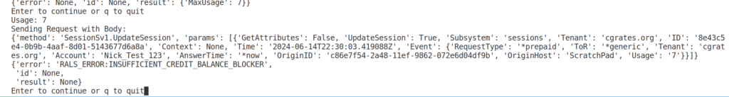
When you run it you’ll be prompted to press enter to continue or input q to quit, let’s enter to continue, then you’ll be asked for the usage, I’ve put 1 in the below example.
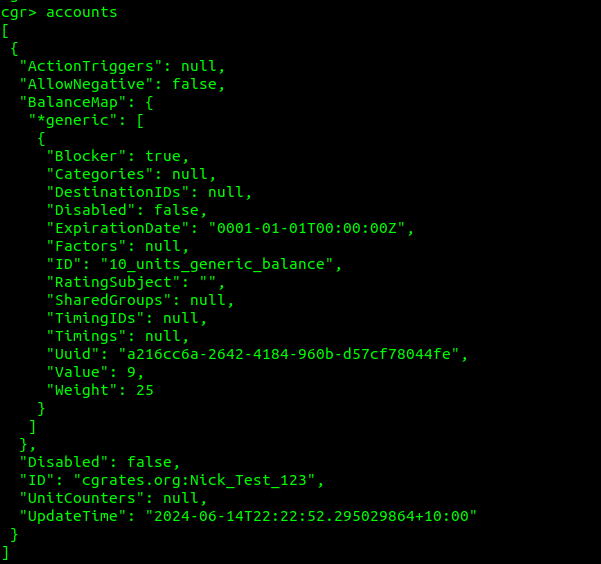
Alright, now let’s take a quick sidebar, and check in with cgr-console in a different tab, what do we think is going to show as our balance?
Well, if we run the accounts command from within cgr-console we can see our account which had a balance of 10 before, now has a balance of 9, as we’ve deducted 1 from the balance by inputting it as our usage:
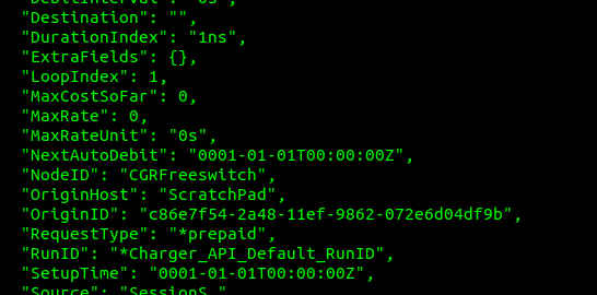
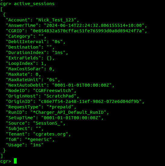
And if we run the active_sessions command in the same console, we see the active sessions, where we can see where that one unit of balance went.
A few things to call out here:
The DebitInterval is how often this balance will be deducted, for our test scenario we’ve turned off automatic debiting, but Agents like FreeSWITCH and Kamailio leave this on and automatically tick off time as it passes (Obliviously this doesn’t work for data, so we’d leave it off)
The LoopIndex is how many UpdateSessions events the API has handled for this session (the unique session is identified by the ID / CGRID field)
SetupTime is blank because we didn’t set it in our initial UpdateSession API Call
The Usage in cgr-console is sometimes shown as nanoseconds, that’s because 1ns is equal to 1 generic unit.
So let’s go back to our Python script, go through the loop again but this time set the usage to 7.
Now if we flip back to cgr-console and check again, we’ll see, as expected that our account balance is now 2, and the active session has 8 of usage.
That’s because we started with 10, then we deducted 1, then we deducted 7, gives us 2 remaining. If we’re to run active_sessions again at cgr-console we’ll see the Usage of the session is now 8.
And lastly let’s try and take another 7 of balance, knowing we’ve only got 2 units left.
No dice; 7 is greater than 2 of course, so CGrateS stops us there by rejecting the request with RALS_ERROR:INSUFFICNET_CREDIT_BALANCE_BLOCKER – SessionS has done it’s job of making sure we didn’t allocate more of the credit than we were allowed and told us we have insufficient credit and that this balance is a blocker.
In this little demo we had one service drawing on the same source, but imagine if you’d fired up two copies of the script, you could have those two sources both consuming data at the same time, and this is where CGrateS shines; CGrateS can do all the heavy lifting to make sure that the resources are never over allocated, and that we’re not ending up with a negative balance.
When it comes time to terminating the session, there’s a trick to this.
Unit reservation is all about allocating resources in advance, this means we’ve generally have taken more money from the balance than we actually ended up consuming, so we have to give this back to the customer.
If we include the Usage field in the TerminateSession request, this must be the total usage for the entire session (start-to-finish), not just since the last UpdateSession API call.
For example if we allocated 30 seconds balance at the start of a call, then as that 30 seconds was consumed, we allocated another 30 seconds, and then when the call got 60 seconds in, we allocate another 30 seconds of balance. But if the call ends at a total of 70 seconds, we’ve allocated 90 seconds (3x 30 seconds), so we’d be over billing the customer. This is where we set Usage to 70 and CGrateS will refund the 20 seconds of balance we over charged them. This is because 3x 30 seconds = 90 seconds allocated, but the call only ended up using 70 seconds, so we need to refund 20 seconds of balance (90 – 70 = 20) to the Account balance.
That’s one way of doing it, but the other option is if we’ve just tracked usage since the last update, we have a 70 second call that we had allocated 3x 30 seconds Session Updates, we can set LastUsed to be 10 seconds (as we only used 10 seconds of the 30 seconds allocated in the last Update) which will also refund the 20 seconds.
In practice, you’ll probably use CGrateS Agents like the FreeSWITCH Agent, Asterisk Agent or Kamailio Agent to handle the charging in those applications. By using the premade CGrateS Agents, it handles generating the UpdateSession calls and all of this logic under the hood, but it’s super useful to know how it all works.
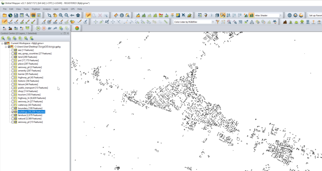
Having building footprints inside Atoll is super-duper valuable, this means you can calculate your percentage of homes / buildings covered, after all geographic coverage and population coverage are two very different things.
Once you’ve got the export, we’ll load the .gpkg file (or files) into GlobalMapper
Select one layer at a time that you want to export into Atoll. (This also works for roads, geographic boundaries, POIs, etc)
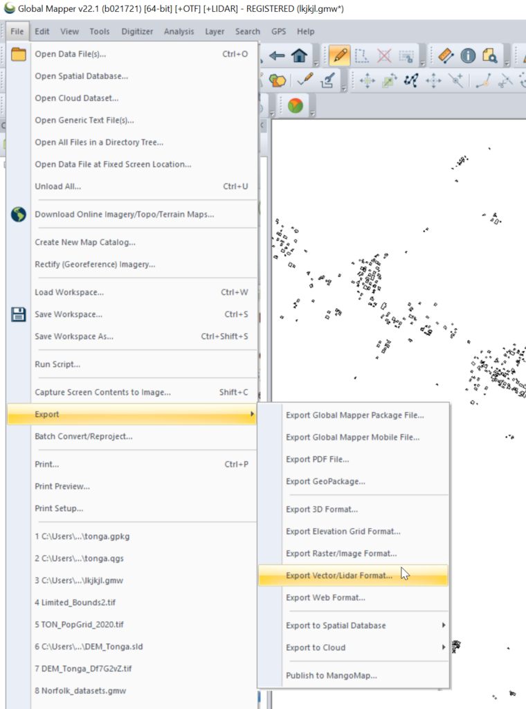
Export the selected layer from Export -> Export Vector / Lidar Format
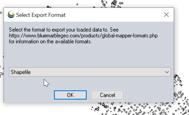
Set output type to “Shapefile”
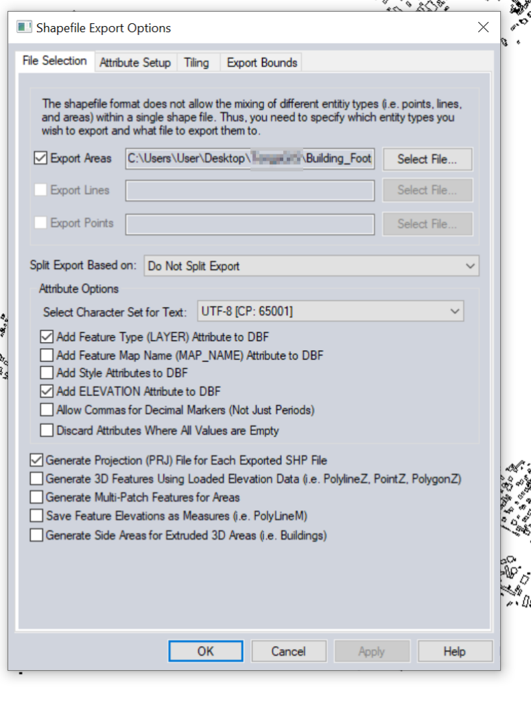
Set output filename in “Export Areas” (This will be the output file). If you want to limit the export to a given area you can do that in Export Bounds.
Now we can import this data into Atoll.
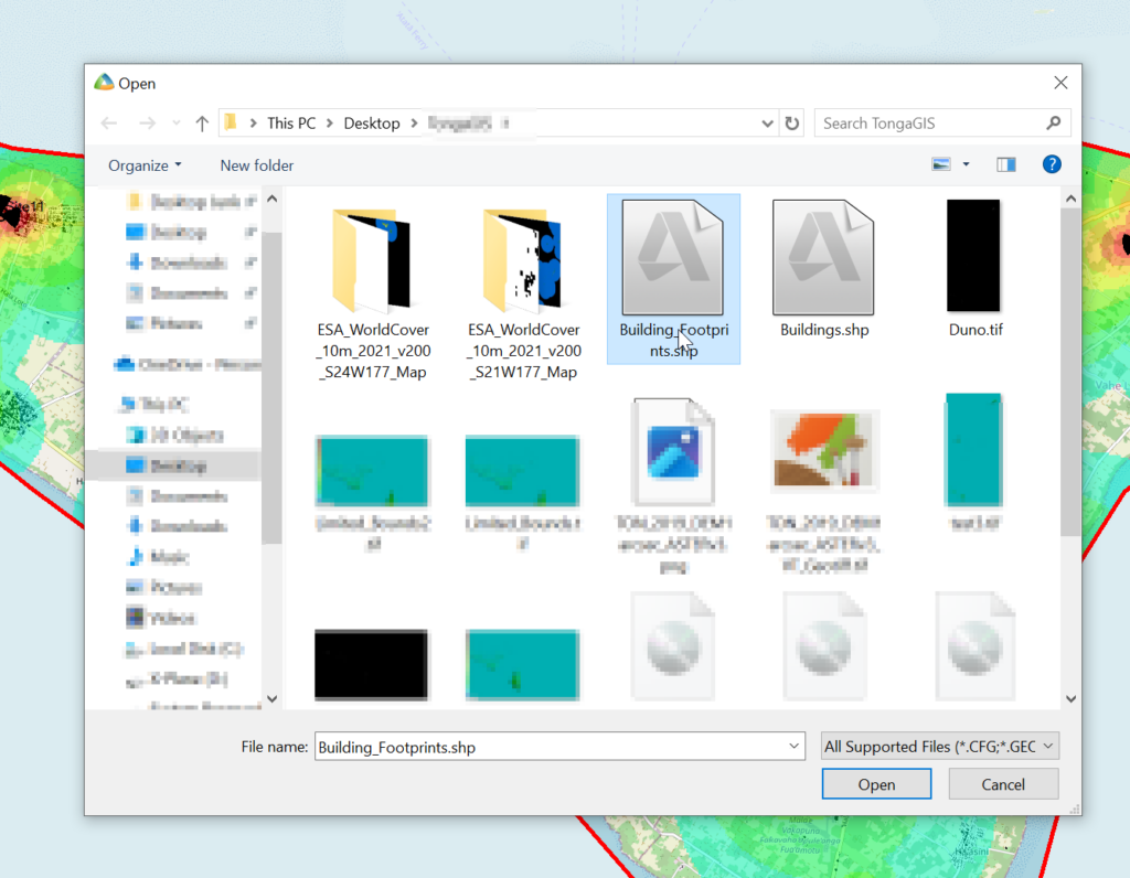
File -> Import
Select the exported Shapefile we just created.
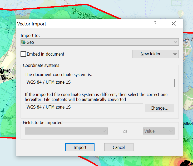
Set the projection and import
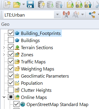
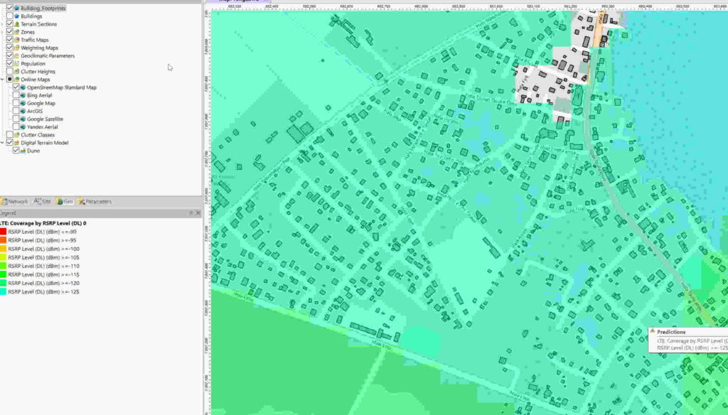
Bingo now we’ve got our building footprints,
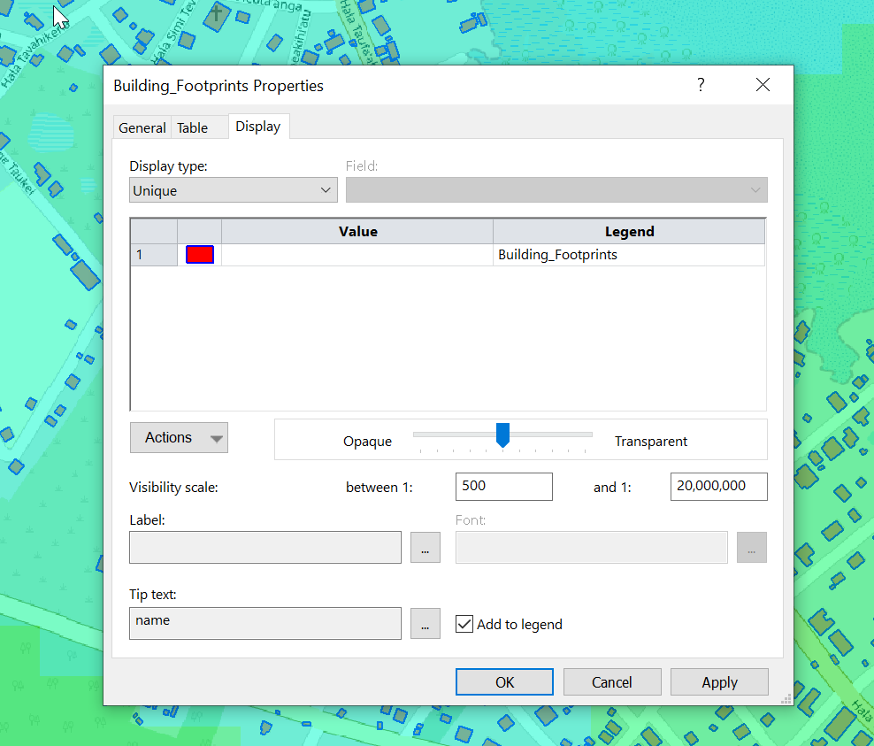
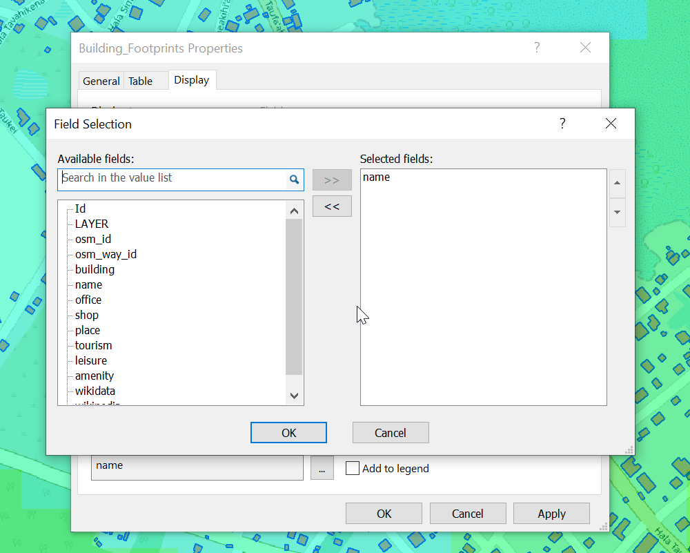
We can change the style of the layer and the labels as needed.
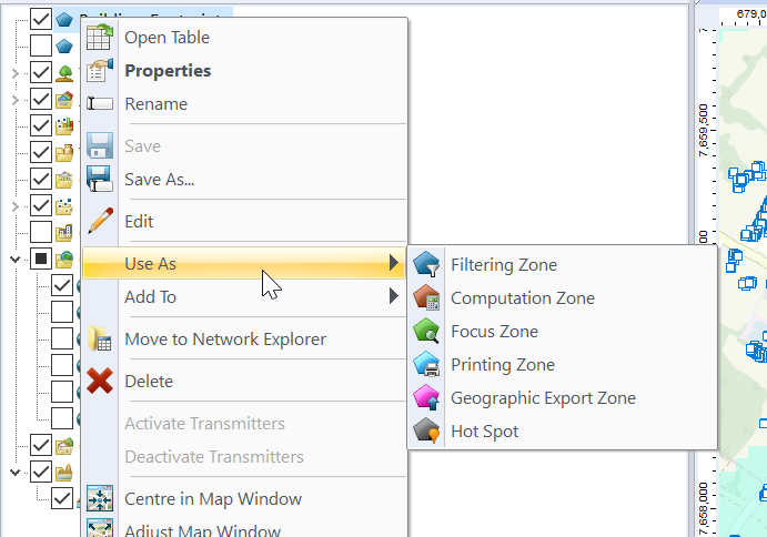
Now we can use the buildings as the Focus Zone / Compute Zone and then run reports and predictions based on those areas.
For example I can run Automatic Cell Planning with the building layers as the Focus zones, to optimize azimuths, tilts and powers to provide coverage to where people live, not just vacant land.
Clutter data describes real world things on the planet’s surface that attenuate signals, for example trees, shrubs, buildings, bodies of water, etc, etc. There’s also different types of trees, some types of trees attenuate signals more than others, different types of buildings are the same.
Getting clutter data used to be crazy expensive, and done on a per country or even per region basis, until the European Space Agency dropped a global dataset free of charge for anyone to use, that covered the entire planet in a single source of data.
So we can use this inside Forsk Atoll for making our predictions.
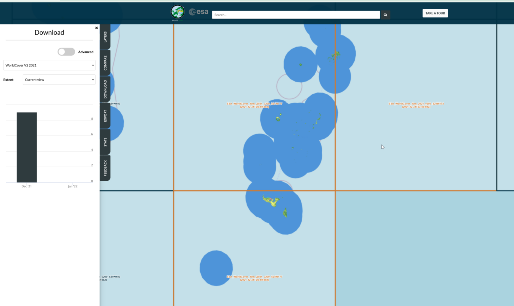
First things first we’ll need to create an account with the ESA (This is not where they take astronaut applications unfortunately, it just gives you access to the datasets).
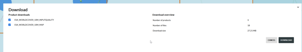
Then you can select the areas (tiles) you want to download after clicking the “Download” tab on the right.
We get a confirmation of the tiles we’re download and we’ll get a ZIP file containing the data.
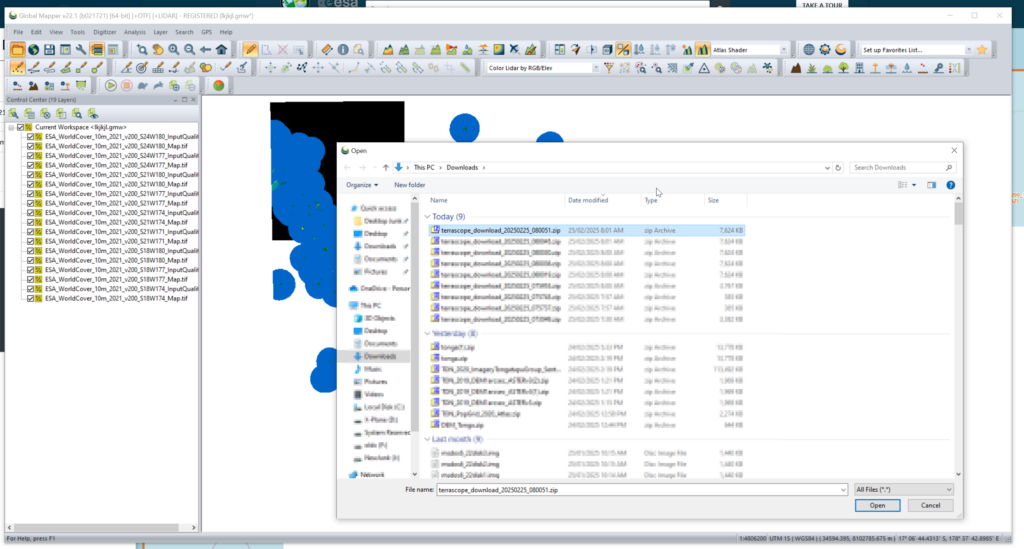
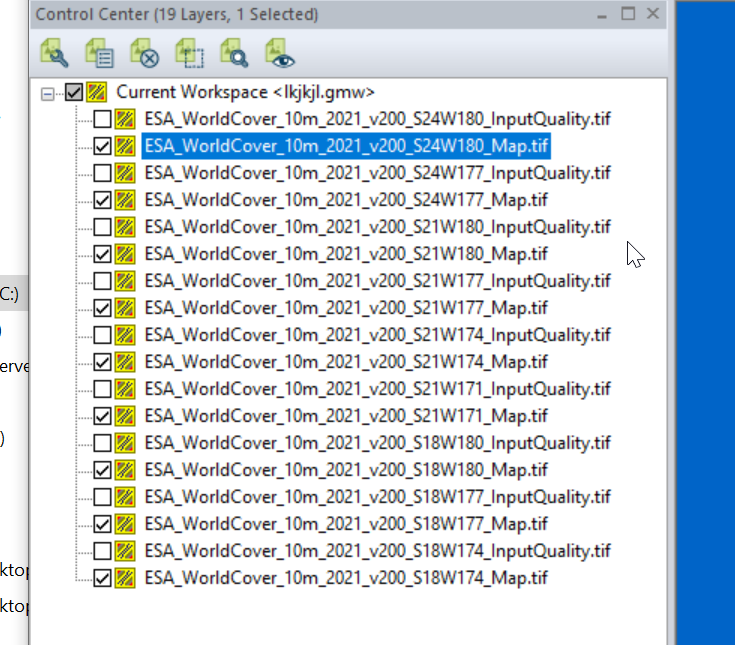
We can load the whole ZIP file (Without needing to extract anything) into GlobalMapper which loads all the layers.
I found the _Map.tif files the highest resolution, so I’m only exporting these.
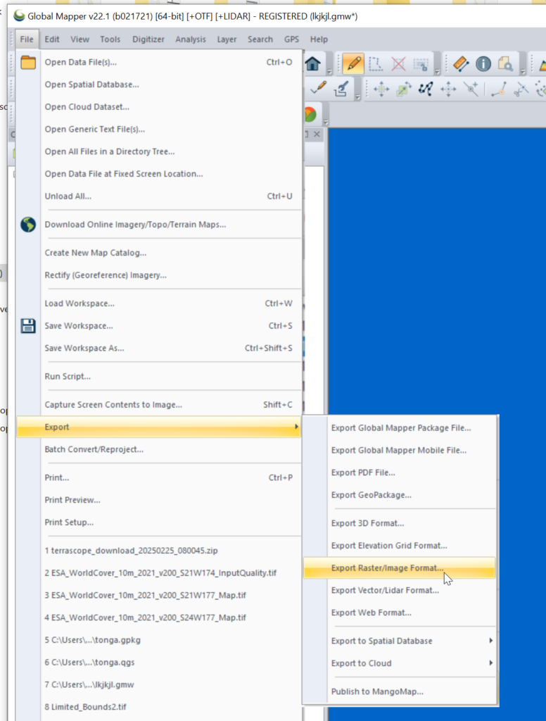
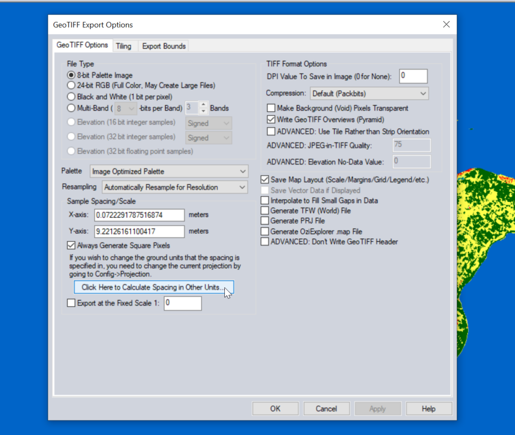
Then we need to export the data to GeoTiff for use in Atoll (The specific GeoTiff format ESA produces them in is not compatible with Atoll hence the need to convert), so we export the layers as Raster / Image format.
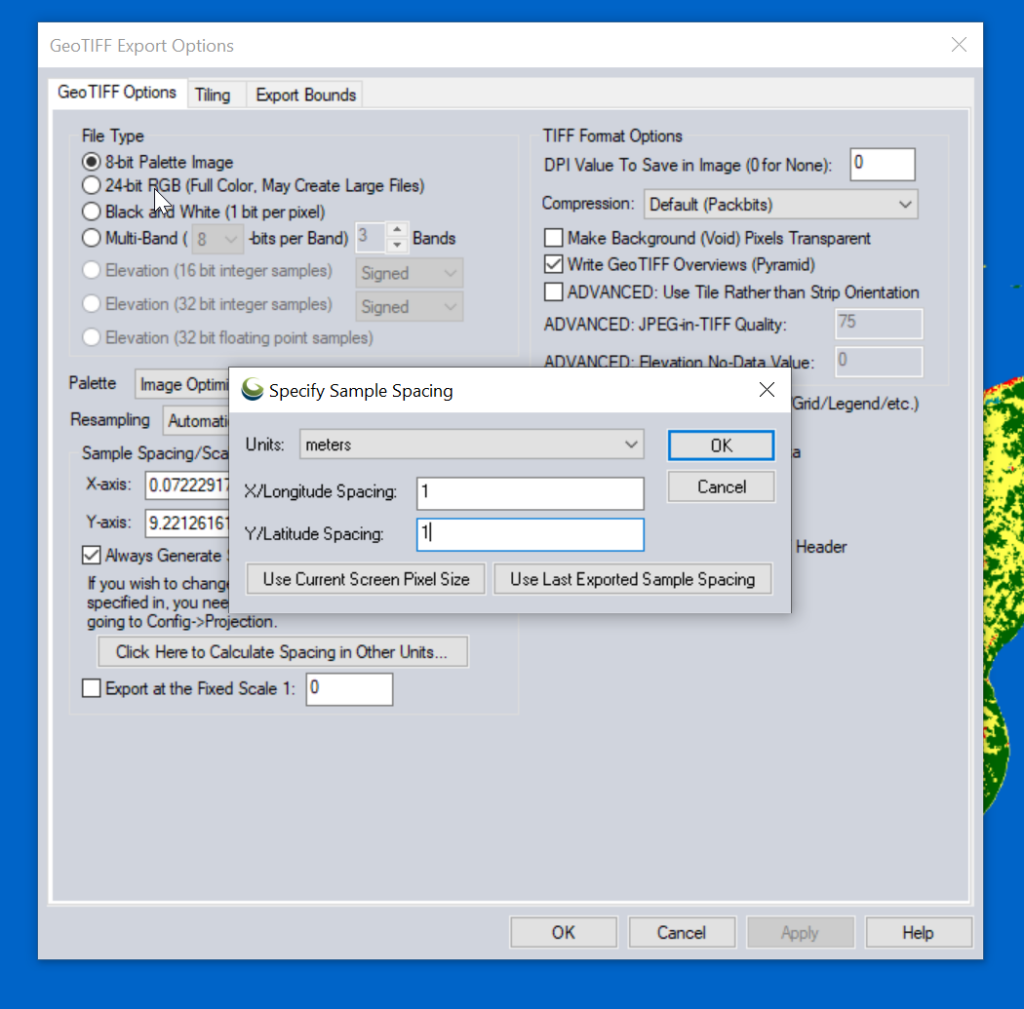
Atoll requires square pixels, and we need them in meters, so we select “Calculate Spacing in Other Units”.
Then set the spacing to meters (I use 1m to match everything else, but the data is actually only 10m accurate, so you could set this to 10m).
You probably want to set the Export Bounds to just the areas you’re interested in, otherwise the data gets really big, really quickly and takes forever to crunch.
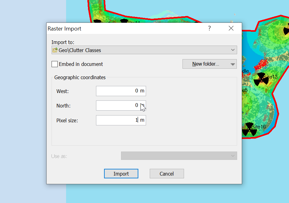
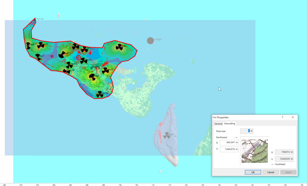
Now for the fancy part, we need to import it into Atoll.
When we import the data we import it as Raster data (Clutter Classes) with a pixel size of 1m.
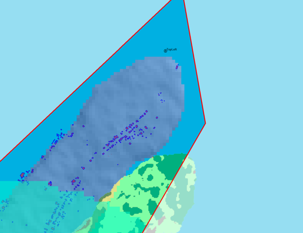
Alas when we exported the data we’ve lost the positioning information, so while we’ve got the clutter data, it’s just there somewhere on the planet, which with the planet being the size it is, is probably not where you need it.
So I cheat, I start put putting the West and North values to match the values from a Cell Site I’ve already got on the map (I put one in the top left and bottom right corners of the map) and use that as the initial value.
Then – and stick with me, this is very technical – I mess with the values until the maps line up into the correct position. Increase X, decrease Y, dialing it it in until the clutter map lines up with the other maps I’ve got.
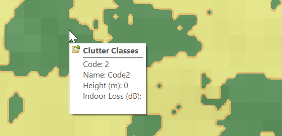
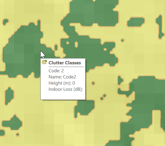
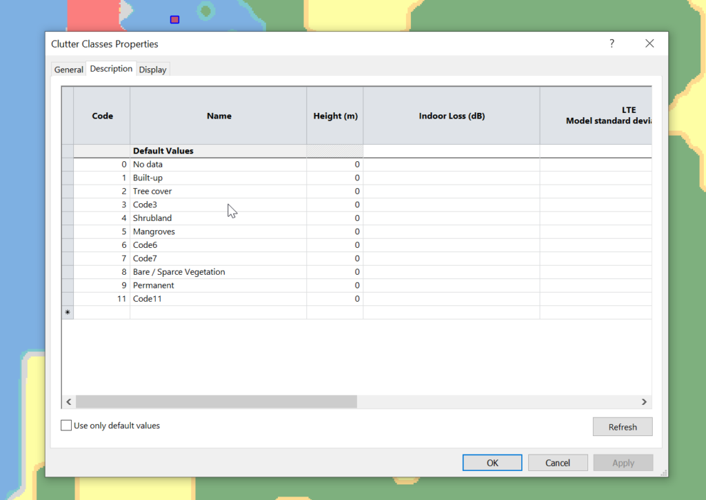
Right, now we’ve got the data but we don’t have any values.
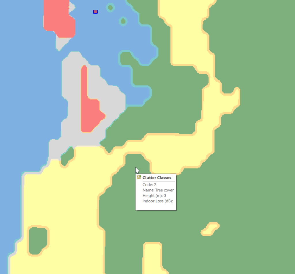
Each color represents a clutter class, but we haven’t set any actual height or losses for that material.
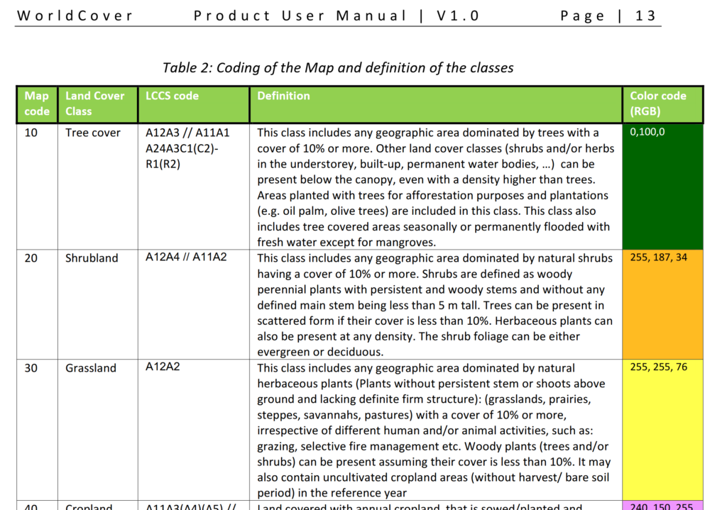
Alas the Map Code does not match with the table in the manual, but the colours do, here’s what mine map to:
Which means when hovering over a layer of clutter I can see the type:
Next we need to populate the heights, indoor and outdoor losses for that given clutter. This is a little more tricky as it’s going to vary geography to geography, but there’s indicative loss numbers available online pretty easily.
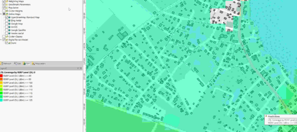
Once you’ve got that plugged in you can run your predictions and off you go!
Another post in the “vendors thought Java would last forever but the web would just a fad” series, this one on getting Nokia BTS Site Manager (which is used to administer the pre-Airscale Nokia base stations) running on a modern Linux distro.
For starters we get the installers (you’ll need to get these from Nokia), and install openjdk-8-jre using whichever package manager your distro supports.
Once that’s installed, then extract the installer folder (Like BTS Site Manager FL18_BTSSM_0000_000434_000000-20250323T000206Z-001.zip).
Inside the extracted folder we’ve got a path like:
BTS Site Manager FL18_BTSSM_0000_000434_000000-20250323T000206Z-001/BTS Site Manager FL18_BTSSM_0000_000434_000000/C_Element/SE_UICA/Setup
The Setup folder contains a bunch of binaries.
We make these executable:
chmod +x BTSSiteEM-FL18-0000_000434_000000*
Then run the binary:
sudo ./BTSSiteEM-FL18-0000_000434_000000_x64.bin
By default it installs to /opt/Nokia/Managers/BTS\ Site/BTS\ Site\ Manager
And we’re done. Your OS may or may not have built a link to the app in your “start menu” / launcher.
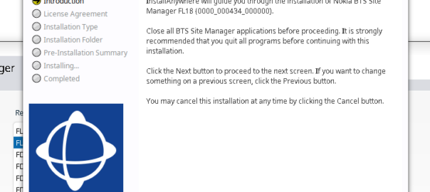
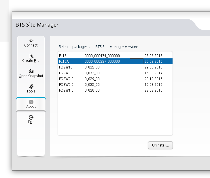
You can use one BTS manager to manage several different versions of software, but you need the definitions for those software loaded.
If you want to load the Releases for other versions (Like other FLF or FL releases) the simplest way is just to install the BTS site manager for those versions and just use the latest, then you’ll get the table of installed versions in the “About” section that you can administer.
Turns out it was great training for a career in telecom; I learned basic rigging, working at heights, electrical work, patching rats nests of cables and the shared camaraderie that comes from having stayed up all night working on something no one would ever notice, unless you hadn’t done it.
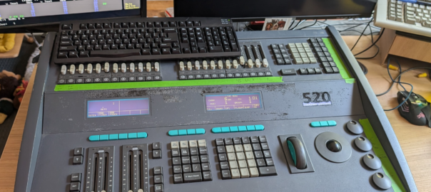
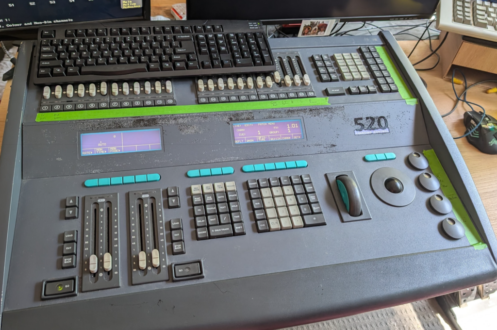
At the time the Strand 520i lighting console was the coolest thing ever, it had support for 4 DMX universes (2048 channels – Who could ever need more than that!?) and cost more than a new car.
One late Friday night browsing online I found one for sale by a University in the state I live in, for $100 or best offer. You better believe I smashed the buy now button so hard my mouse almost broke. I was going to own my very own Strand 520.
I spent the weekend reading through the old manuals, remembering how to use all the features, then dragged my partner for the road trip the following Monday morning to pick it up and bring it home.
But before I could do anything fun I had to find a PS/2 keyboard and a VGA screen, which took me a few more days (a visit to the tip was the easiest way to get a hold of them).
Then I needed something to receive DMX – I found everything now uses ArtNet (DMX over IP) and there’s visualisers for simulating an arena / stage lighting setup, but all take ArtNet now, so I ordered a DMX to ArtNet converter.
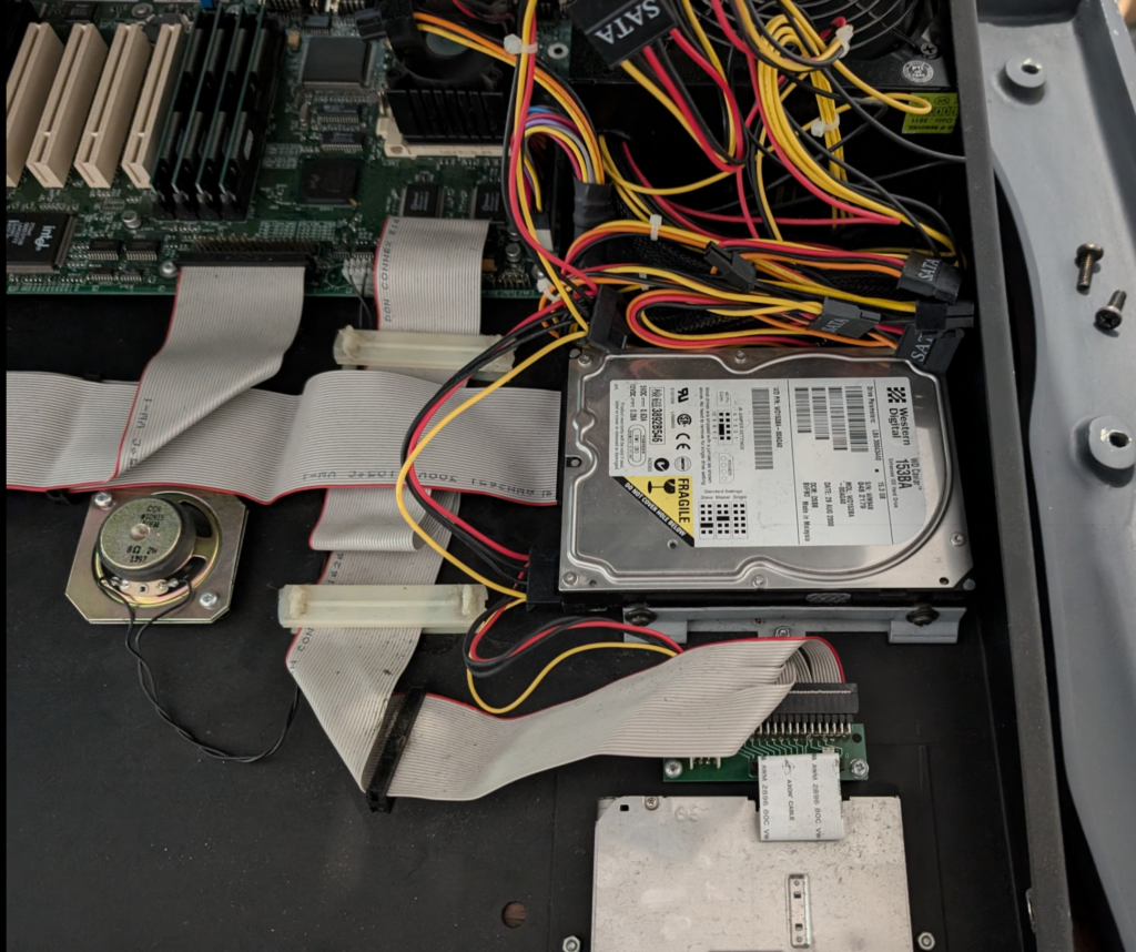
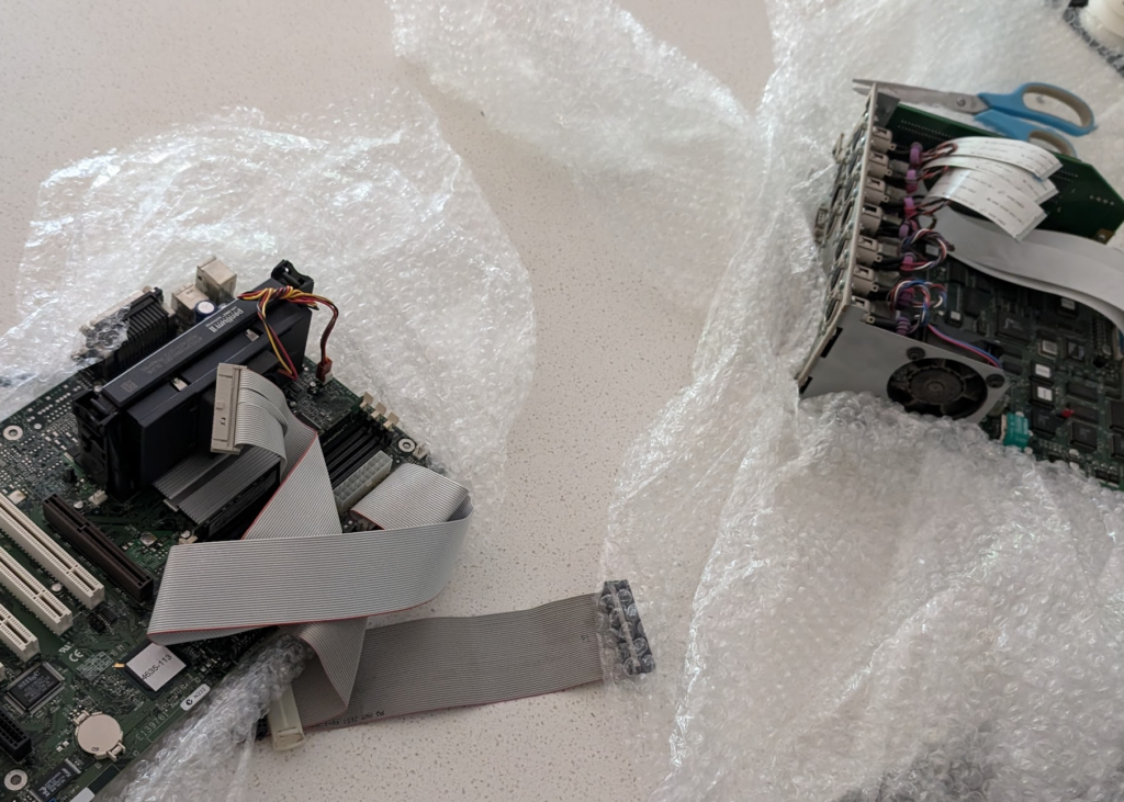
Inside the unit is pretty much a standard PC (An “OG” Pentium in the Strand 520) with an ISA card for all the lighting control stuff.
The clicking hard drive managed to boot, but I didn’t think it’d last long, having been made more than 25 years prior. So I created a disk image and copied the file system onto a CF card using a CF to IDE adapter. This trick meant it booted faster than ever before.
Clicky HDD before it became a CF
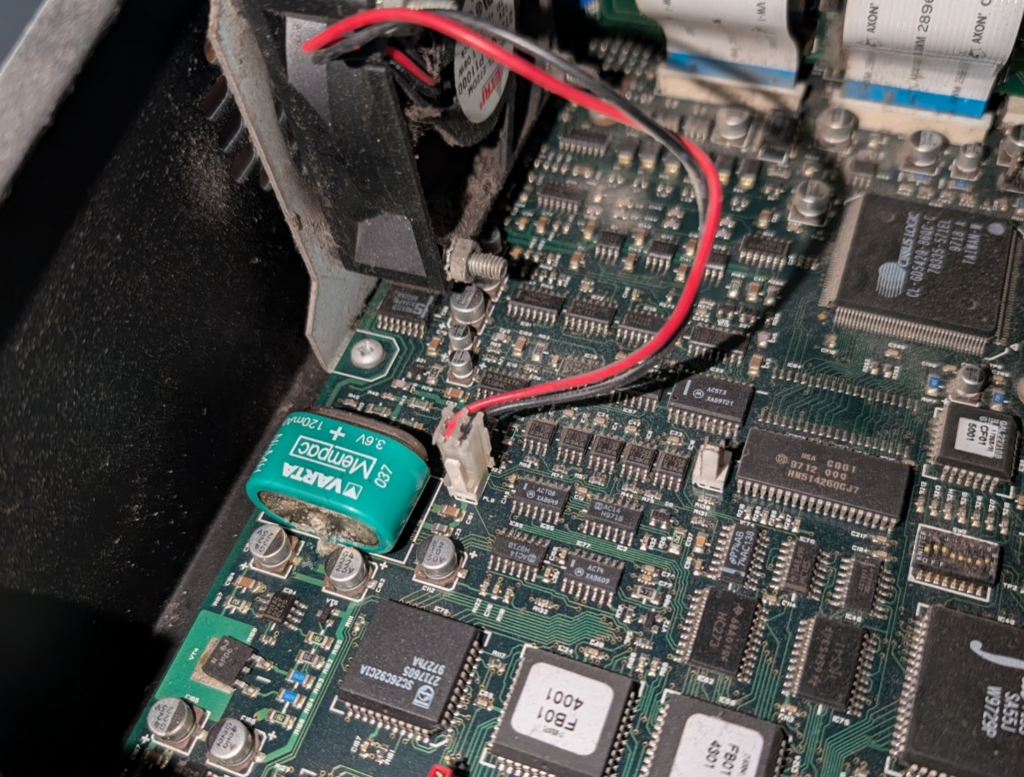
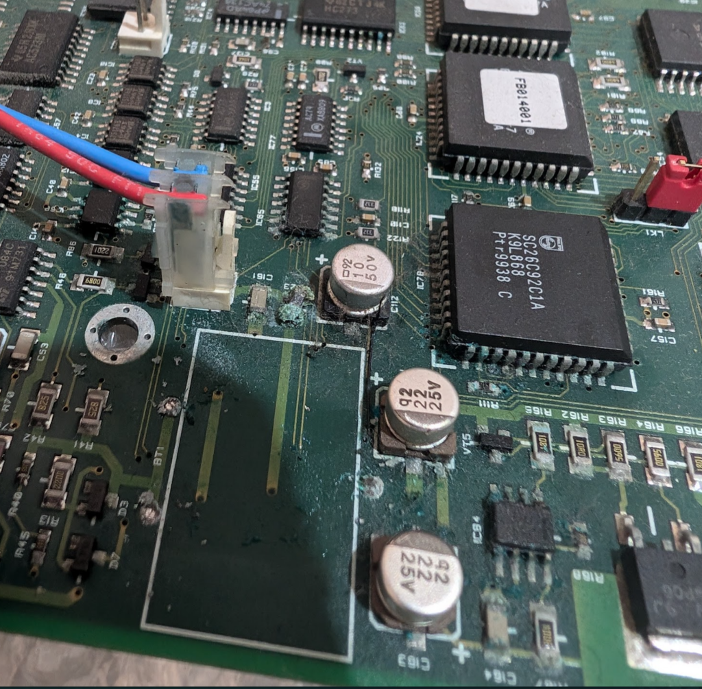
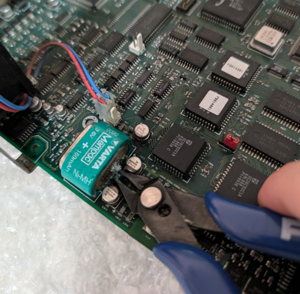
One thing I’d read about online was the VARTA battery had a tendency to leak battery acid all over the PCB. This one had yet to fully spill its guts, but was looking a bit bulgey and had started to leak a little already.
The battery (I’d read) was only for storing info in a power loss scenario, and if the battery isn’t present it just slows the boot time as everything has to be read from disk, so I took the leap of faith and cut the battery out, and lo, it still all boots.
Slightly furry VARTA battery
So now I was OK to get the desk online properly, but was getting semi-regular lock ups where DMX would stop outputting and inputs on the console were not read, but the underlying PC was still working.
I spent a lot time debugging this. BIOS settings, interrupts, I dived into how ISA works, replaced the battery I removed with a brand new one, and at one point I broke out the oscilloscope, but nothing worked.
Around the same time I noticed the Ethernet port (BNC!) would work if I just ran plain DOS (could ping from DOS but when the application started the NIC would go dead), which made me think I may be facing a hardware fault with the “CS” – the show processor for the console which is what the motherboard connects to via ISA.
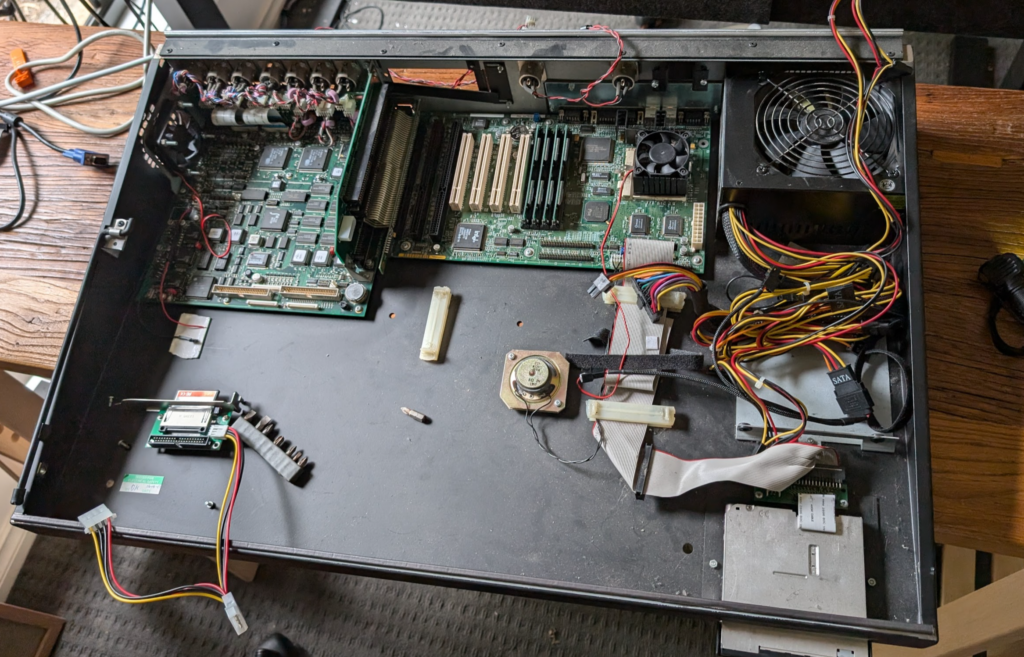
The desk itself with the face off, and the CF adapter being mounted
Alas being almost 30 years old (this unit was made in 1996) there aren’t a great number of them around to test with, so I could try swapping out the “CS” board. What I did find was another complete console on eBay for $50 but it was in the UK, and they weigh a lot. Shipping this thing was not an option.
But for a bit of of extra cash the seller was willing to crack the case open and strip out the two main boards and post me just those. This had added bonus that the motherboard and CPU of the board sent from the UK was a 520i meaning it has the Pentium II processor – This Strand 520 was now going to be a Strand 520i.
A month later a box appeared at my door containing the boards, but the battery on the CS board from the UK had well and truly spilled its guts, leaving some toxic sludge around all the components nearby. A can of PCB cleaner and a toothbrush (which I will not be using to brush teeth with anymore) and I’d cleaned it up as best I could, but the fan output from the board was well and truly dead, with some of the SMD components just eaten by the acid.
So I put everything back into the case and wired it up. The mounts for the Motherboard were slightly different, and the software that is used for the 520i is different from the 520 (without the i).
The HDD from the UK was unable to boot, but I was able to get it to spin up enough to copy off the ~5Mb of files I needed, then I did a fresh install of MS DOS and copied the installer for the StrandOS.
Finally fully functional
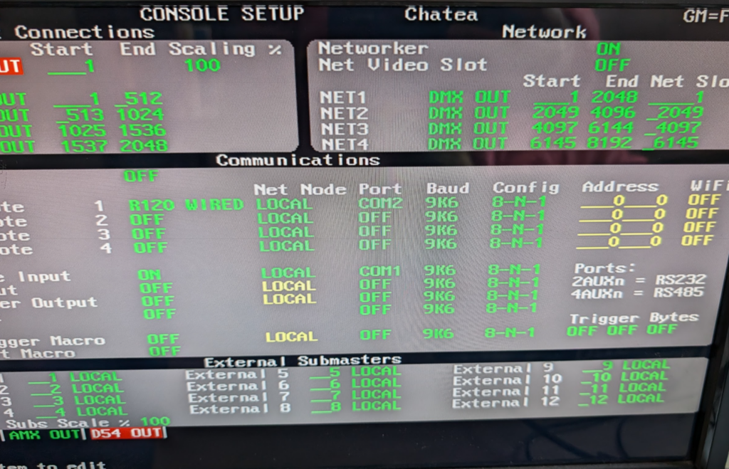
Finally I had a stable working console. Not just that but the Strand Networker application was now available to me. So I plugged into the 10Mbps connection and set the console to output to Network as well as DMX.
Enabling the “networker” for network DMX transmission
I cranked open Wireshark and there was a mystery signal sent to the broadcast address on UDP…
I patched a single DMX channel and changed the value and when I viewed the data in Wireshark I could see a hex representation of the DMX 0-255 value.
Easy I thought to myself, it’ll just be a grid of channels, each with their value as hex. Ha! I was wrong.
Turns out Strand Shownet used a conditional form of “Run Length Encoding” compression, where if you’ve got channels 1 through 5 at 50% rather than encoding this is 5 bytes each showing 0x80, it uses 2 bytes, to indicate 5 sequential channels (run length) and then the value (0x80). Then there’s another bit to denote how many forward places to move and if the next channel is using RLE or not.
The code got messy; it’s not the best thing I’ve ever written but it works for 2 full universes of DMX (I need to spend more time to understand where the channel encoding overflow happens as I end up a few channels ahead of where I should be on universe 3 and above).
The code is available on Github and I’d love to know if anyone’s using it with these old dinosaurs!
I love Grafana. I love metrics and observability. Nothing is more powerful than being able to see what’s going on inside your network/application/solar setup/weather station – you name it.
It’s never been easier to see what’s going on.
If I wanted to monitor my web app as I onboard more customers, Grafana is the go-to tool, but how was it done before the computer age? Let’s go back to the 1940s and look at how the telephone network handled observability and metrics…
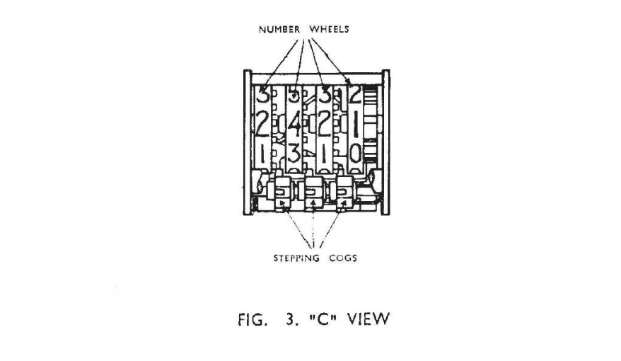
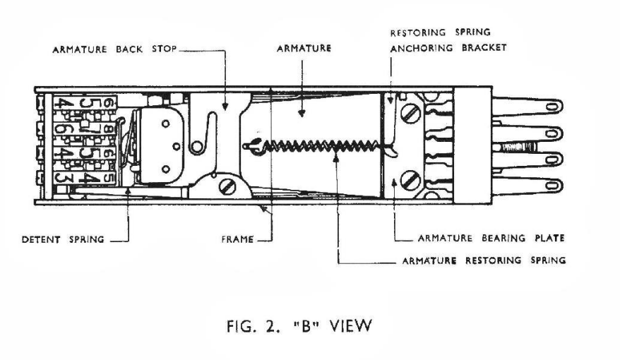
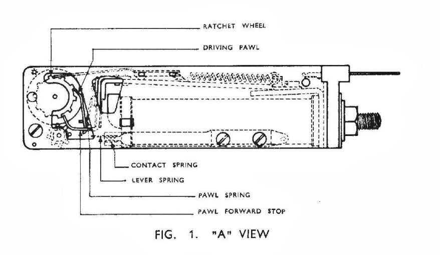
This starts with introducing the “Call Meter”, “Subscriber Meter” or “Subs Meter” for short.
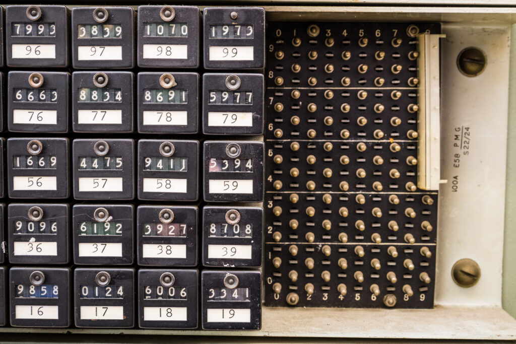
Detail of mechanical call meter Strathfield South Exchange Source – field, field, field and chang’s brilliantly beautiful “That Exchange Project“
The concept is pretty simple. Each telephone service (“subscriber” in telecom parlance) provided by the local telephone exchange gets a subscriber meter or “subs meter”.
When the subscriber (customer) makes a call, and the call is answered, a reverse of polarity on the line ticks the subscriber meter over by one digit.
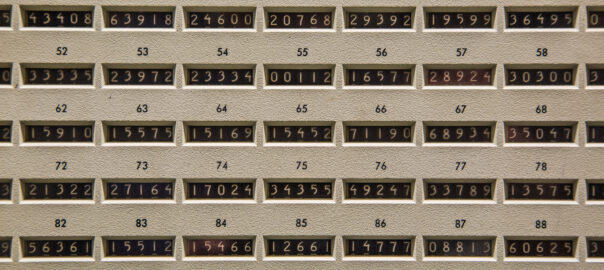
Each of the meters on the left is a single telephone subscriber, each time they make a call, the meter ticks up by one position. Source – field, field, field and chang’s brilliantly beautiful “That Exchange Project“
As you can imagine if you’ve got a telephone exchange that serves 10,000 customers, well you need 10,000 subscriber meters…
You need a lot of meters… Source – field, field, field and chang’s brilliantly beautiful “That Exchange Project“
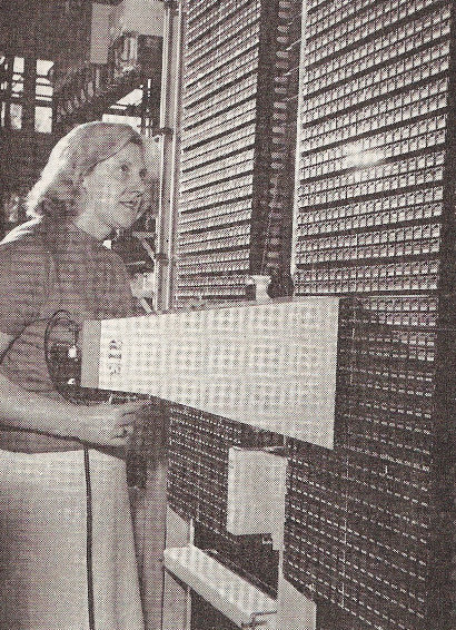
At the end of the month, someone takes a photo of all the meters on a film camera, sends it off to a billing center where they develop the photo, then calculate the difference in values from last month’s meter reading photo and this month’s meter reading photo, and bingo – there’s the number of calls the person made. You tabulate the cost on an adding machine and send off the invoice.
Each of the little blocks is a single subscriber to meter and the weird cone thing held is a hood for the camera to photograph the values – Source The Communications Museum Trust
Optional Sidebar for those asking “but what about Long Distance calls where you pay per minute?” – In a world where you pay per local call, regardless of length, this works just fine, but as more complicated scenarios like long distance calling were introduced, this presented a challenge, but this could be solved by reversing the line polarity at predefined intervals, to keep ticking up the subscriber meters during the call. Exchange Clocks provided a number of pulse outputs, like 1 pulse per second, 1 pulse per minute, etc, this 1 pulse per minute signal could be hooked up to the line reversal circuit for long distance calls, to trigger the line reversal every minute. This means if a local call was $0.40 untimed, if you made long distance calls at $0.40 per minute, then you just needed the exchange to reverse the line every minute to pulse the meter. 10 increments on the meter could mean 10 x $0.40 local calls or 10 minutes of $0.40 per minute long distance.
These meters were originally just for metering traffic, but engineers in the telephone network realised they could be used as generic “counters” for just about anything in the telephone network.
Let’s imagine you want to know how often a trunk line to another exchange runs out of capacity, well, you simply wire a meter to get triggered each time that condition happens, now you’ve got a counter for each time that event occurs.
Now let’s say you want to know how often you run out of final selectors, well, through another counter on it.
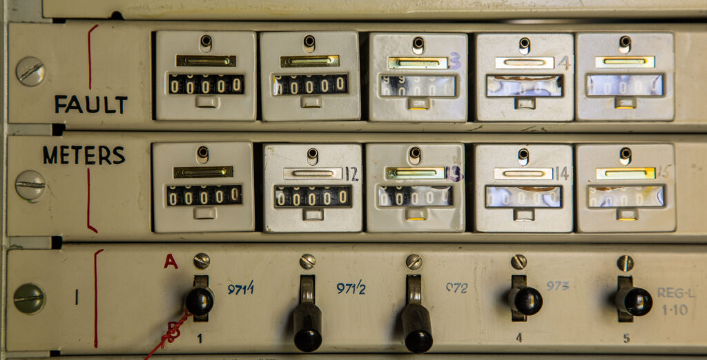
These same meters, can be wired to count fault conditions.
Mechanical fault meters on old step-by-step test desk, Queanbeyan Exchange Source – field, field, field and chang’s brilliantly beautiful “That Exchange Project“
A pencil and a logbook is how you keep track of frequency of the event being triggered, and if you want to graph it out, graph paper, not Grafana.
As telephone systems increased in complexity more and more meters were used to track what’s going on, up until the time that computers could start to handle that process, when “Electronic Customer Metering” came into play with the early Stored Program Control exchanges.
Metering and charging equipment in Blakehurst Exchange Source – field, field, field and chang’s brilliantly beautiful “That Exchange Project“
Observability and Metrics are so important for making software, but every time I define a “counter” in software for an event, I’m always reminded of clicking meters in an telephone exchange, knowing this is how it used to be done.
Last year we deployed some Hughes HL1120W OneWeb terminals in one of the remote cellular networks we support.
Unfortunately it was failing to meet our expectations in terms of performance and reliability – We were seeing multiple dropouts every few hours, for between 30 seconds and ~3 minutes at a time, and while our reseller was great, we weren’t really getting anywhere with Eutelsat in terms of understanding why it wasn’t working.
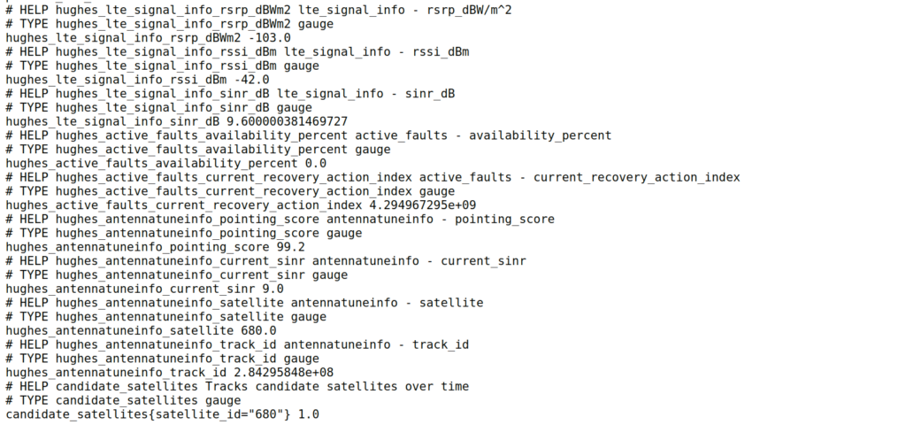
Luckily for us, Hughes (who manufacture the OneWeb terminals) have an unprotected API (*facepalm*) from which we can scrape all the information about what the terminal sees.
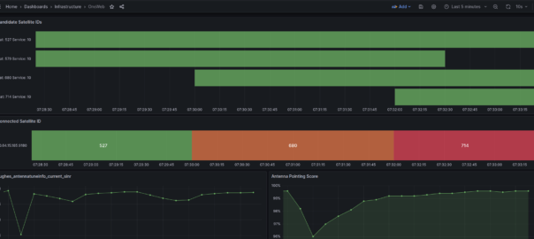
As that data is in an API we have to query, I knocked up a quick Python script to poll the API and convert the data from the API into Prometheus data so we could put it into Grafana and visualise what’s going on with the terminals and the constellation.
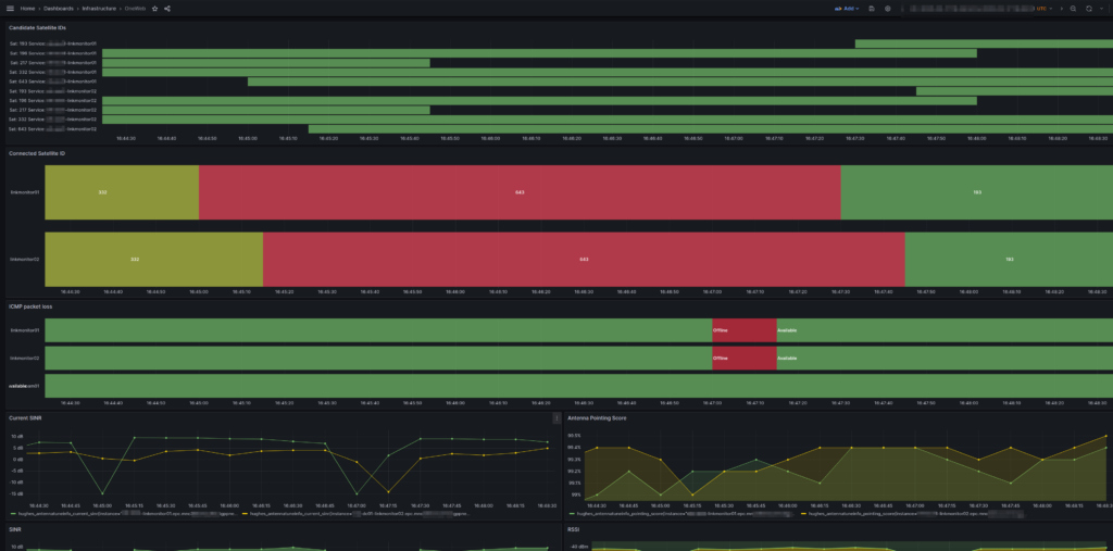
After getting all this into Grafana and combining it with the ICMP Blackbox exporter (we configured Blackbox to send HTTP requests and ICMP pings out of each of the different satellite terminals we had (a mix of OneWeb and others)) we could see a pattern emerging where certain “birds” (satellites) that passed overhead would come with packet loss and dropouts.
It was the same satellites each time that led to the drops, which allowed us to pinpoint to say when we see this satellite coming over the horizon, we know there’s going to be some packet loss.
In the end Eutelsat acknowledged they had two faulty satellites in the orbit we are using, hence seeing the dropouts, and they are currently working on resolving this (but that actually does require rockets, so we’re left without a usable service for the time being) but it was a fun problem to diagnose and a good chance to learn more about space.
Packet loss on the two OneWeb terminals (Not seen on other constellation) correlated with a given satellite pass
The repo has instructions for use and the Grafana templates we used.
At one point I started playing with the OneWeb Ephemeris data so I could calculate the azimuth and elevation of each of the birds from our relative position, and work out distances and angles from the terminal. The maths was kinda fun, but oddly the datetimes in the OneWeb ephemeris data set seems to be about 10 years and 10 days behind the current datetime – Possibly this gives an insight into OneWeb’s two day outage at the start of the year due to their software not handling leap years.
Despite all these teething issues I’m still optimistic about OneWeb, Kupler and Qianfan (Thousand Sails) opening up the LEO market and covering more people in more places.
Update: Thanks to Scott via email who sent this: One note, there’s a difference between GPS time and Unix time of about 10 years 5 days. This is due to a) the Unix epoch starting 1970-01-01 and the gps epoch starting 1980-01-05 and b) gps time is not adjusted for leap seconds, and ends up being offset by an integer number of seconds.
One of the really neat features about using automated RF planning tools like Forsk Atoll is you’re able to get it to automatically try out tweaks and look at how that impacts performance.
In the past you’d adjust something, run the simulation again, look at the results and compare to what you had before,
Atoll’s ACP (Automatic Cell Planning) module allows you to automate this, and in most cases, it does a better job than I would!
Today we’ll look at Cell Site Selection in Atoll.
To begin with we’ll limit the computation area down to a polygon we draw around the area in question,
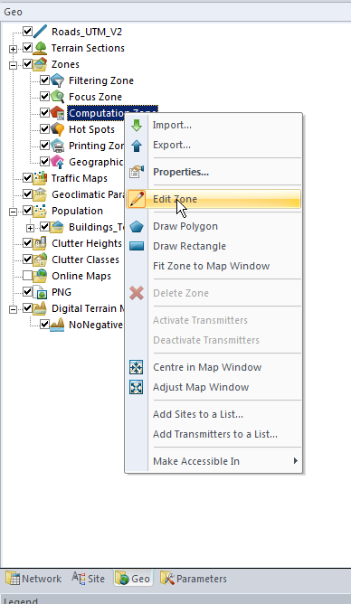
In the Geo tab we’ll select Zones -> Computation Zone and select Edit
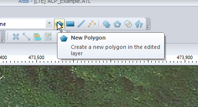
We’ll create a new Polygon and draw around the area we are going to analyze. You can automate this step based on population levels, etc, if you’ve got that data present.
So now we’ve set our computation area to the selection, but if we didn’t do this, we’d be computing for the whole world, and that might take a while…
Generating Candidate Sites
Atoll sucks at this, I’ve found if your computation zone is set, and it’s not a rectangle, bad things happen, so I’ve written a little script to generate candidates for me.
Creating an new ACP Job
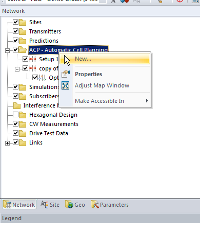
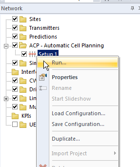
From the Network tab, right click on ACP Automatic Cell Planning and select New
Optimization Tab
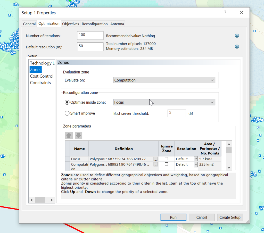
Before we can define all the specifics of what we’re looking to plan / improve, we need to set some limits on the software itself and tell it what we’re looking to improve.
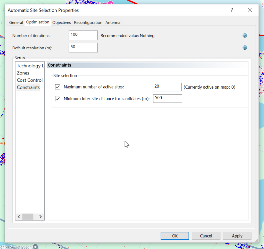
The resolution defines how precise the results should be, and the iterations defines how many changes the software should run through.
The higher the number of iterations, the better the results, but it’s not linear – The improvement between 1000 iterations and 1,000,000,000 iterations is typically pretty minor, and this is because ACP works kind of a “getting warmer” philosophy, where it changes a value up or down, looks at the overall result and then if the result was better, changes the value again until it stops getting better.
As I’m working in a fairly small area I’m going to set 100 iterations and a 50m resolution.
In the optimization tab we can also set constraints, for example we’re looking at where to place cell sites in an area, and as far as Atoll is concerned if we just throw hundreds of sites at an area we’ll have pretty good results, but the economics of that doesn’t work, so we can set constraints, for example for site selection we may want to set the max number of cell sites. As we are importing ~5k candidate locations, we probably don’t want to build 5k cell sites 20m apart, so set this to be a reasonable number for your geography.
When using ACP for Optimization as we can see later on, we can also set cost constraints regarding the cost to make changes, but for now this is just going to pick best cell sites locations for us.
Objectives Tab
Next up we’ll need to setup Automatic Cell Plannings’ objectives.
For ACP to be an effective tool we need to define what we’re looking for in terms of success, you can’t just throw it some values and say “Make it better” – we need to define what parameters we’re looking to improve. We do this by setting Objectives.
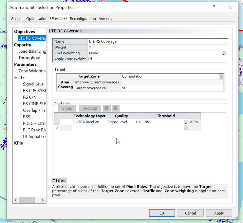
Your objectives are going to be based on your needs and wants, but for this example we’re building greenfield networks, so want to offer coverage over an area, as well as good RSRP and RSRQ, so we will set the objectives to Coverage of 95% of the Computation Zone for this post, with a secondary objective of increasing RSRP and RSRQ.
But today I’m modeling for coverage, so let’s set that:
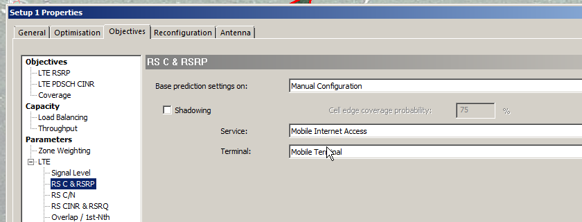
As we’re planning for LTE we need to set the UE parameters, as I’m planning for a mobile network, I’ll need to set the service type and terminal.
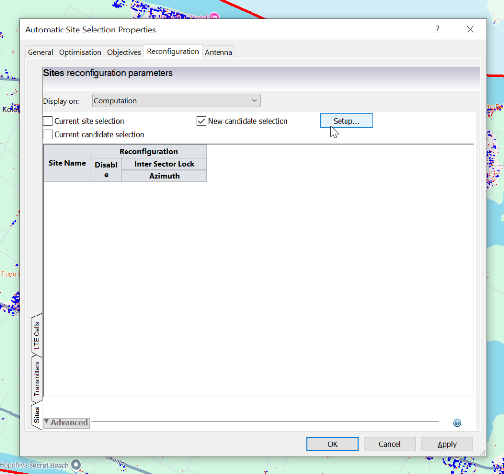
Reconfiguration
Now we’ve defined the Objectives, it’s now time to define what values ACP can mess with to try and achieve these objectives, for some ACP runs you may be adjusting tilts or azimuths, swapping out antennas, etc, but today we’re looking for where we can put cell sites to be the most effective to serve our target area.
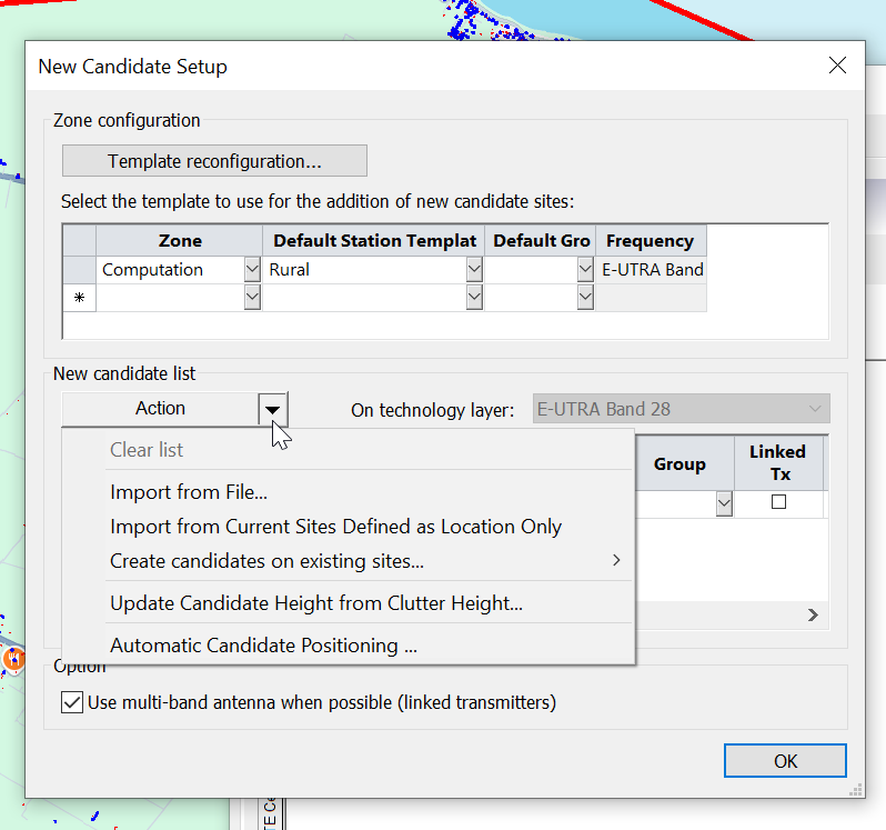
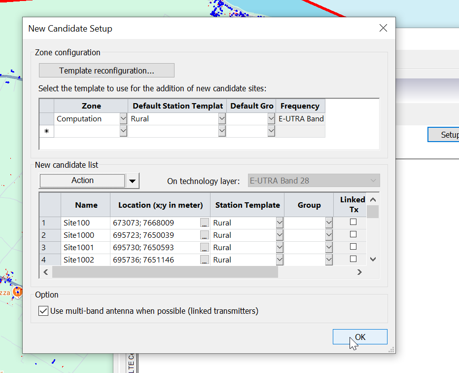
Now we import our candidate list. This might be a list of potential towers you can use, or in my case, for something greenfield, I’m just importing a list of points on a map every X meters to find the best locations to place towers.
From the “Reconfiguration”, we’ll select “Setup” to add the sites we want to evalute.
Atoll has “Automatic Candidate Positioning” which allows it to generate pins on the map, but I’ve not had any luck with it, instead I’m importing a list of candidates I’ve generated via a little Python script, so I’ll select “Import from File”.
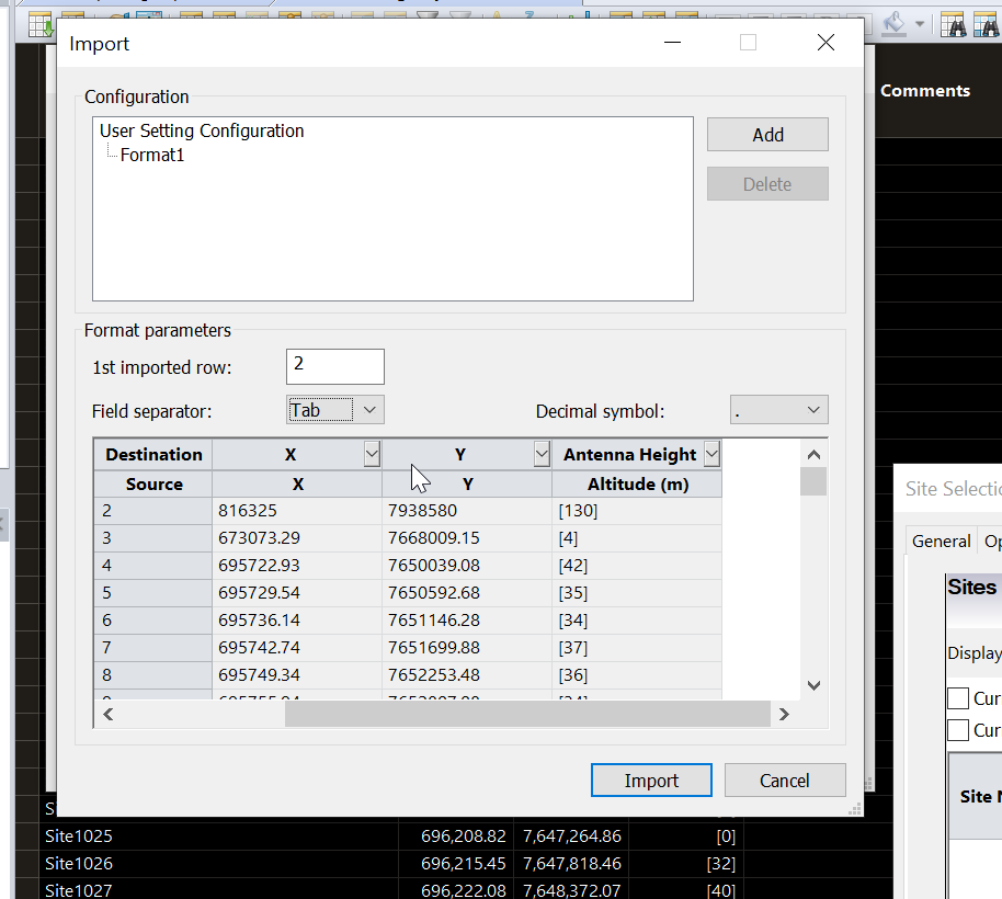
Pick my file and set the parameters for importing the data like so.
Now we’ve got candidates for cell sites defined, we set the station template to populate and then we’re good to go.
Running ACP
Once you’ve tweaked all your ACP values as required, we can run the ACP job,
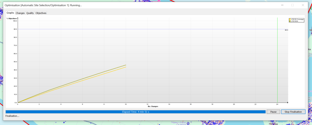
As ACP runs you’ll see a graph showing the objectives and the levels it needs to reach to satisfy them, this step can take a super dooper long time – Especially if your computation zone is large or your number of candidates is large.
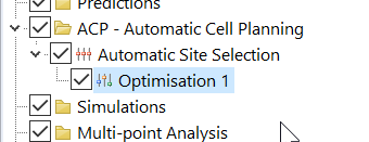
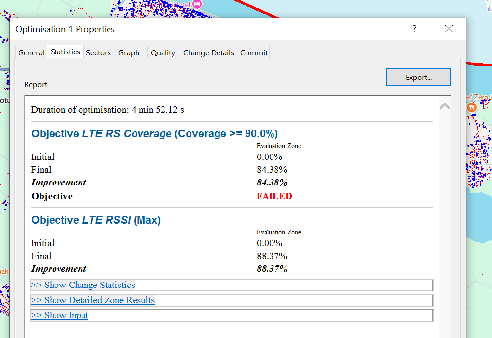
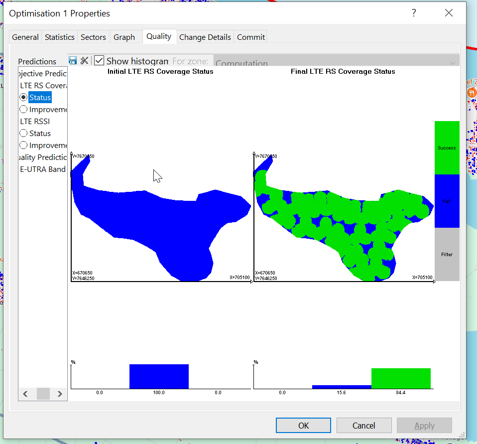
But eventually we’ll be a lot older and wearier, but ACP will have completed, and we can checkout the Optimization it’s created.
In my case the objectives failed to be met, but that’s OK for me,
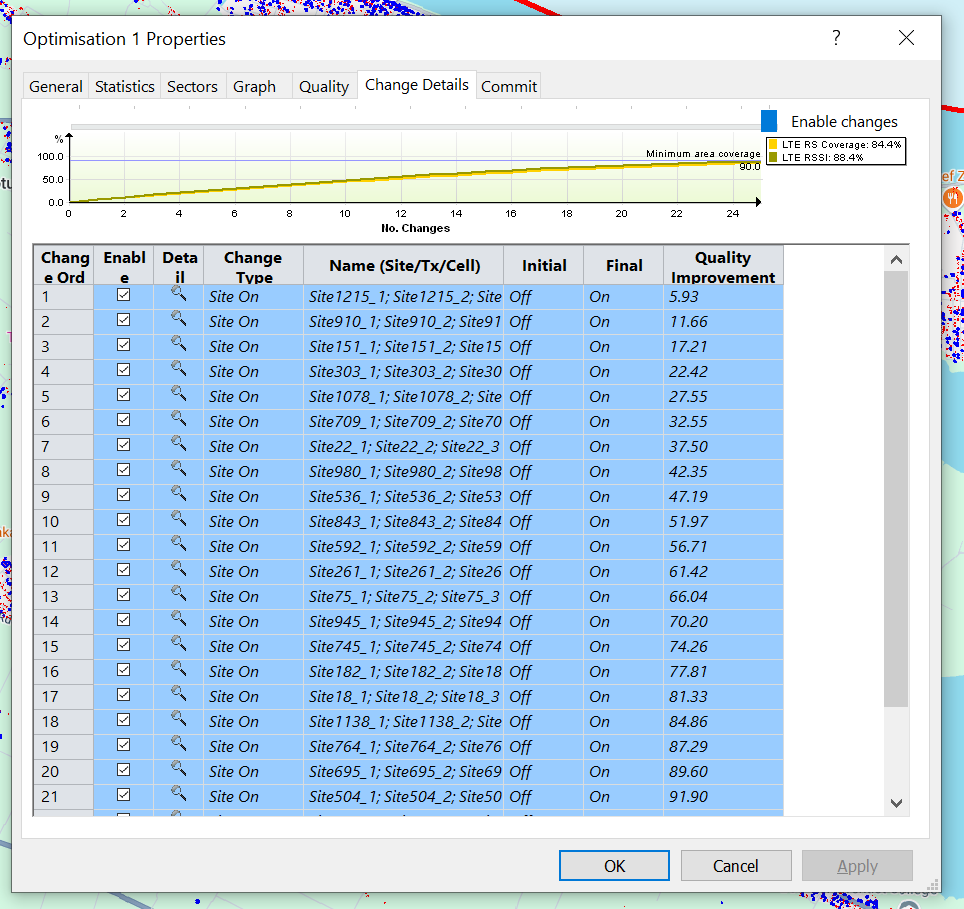
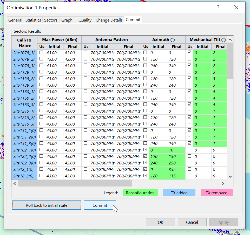
One it’s completed the Changes tab outlines the recommended changes, and the Objectives outlines how this has performed against the criteria we outlined at the start, and if we’re happy with the result, we can Commit the changes to put them on the map from the commit tab.
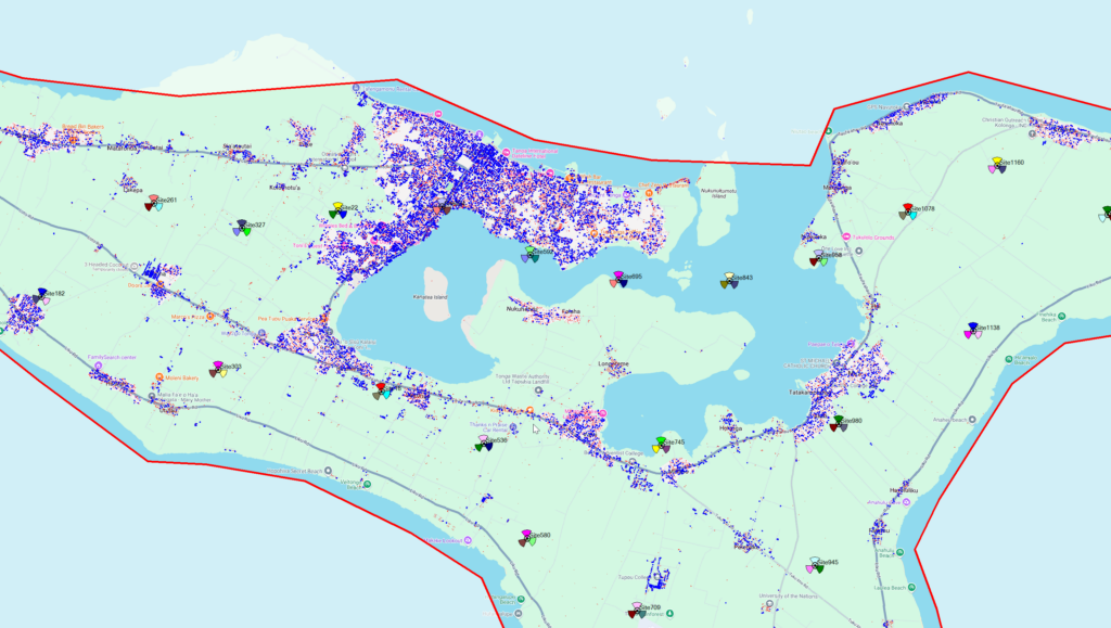
With that done I weed out the sites in impractical locations, the the ones in the sea…
Now we’ve got the sites plugged in, the next thing we’ll start doing is optimizing them.
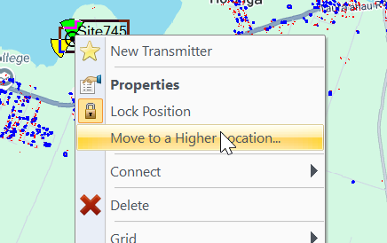
When we’re dealing with greenfield builds like we are today, the “Move to highest location with X Meters” function is super useful. If you’ve got a high point on a property, we want to build our tower on the highest point, so the tower is moved to the highest point.
One thing to note is this just plans our grid. It won’t adjust azimuths, downtilts, etc, in one operation. We need to use another ACP operation to achieve that, and that’s the content of a different post!
The StatS subsystem allows us to calculate statistics based on CGrateS events.
Each StatS object contains one or more “metrics” which are things like Average call duration, Total call duration, Average call cost or totals and average of other fields.
The first thing we’ll need to do is enable stats in our JSON config file:
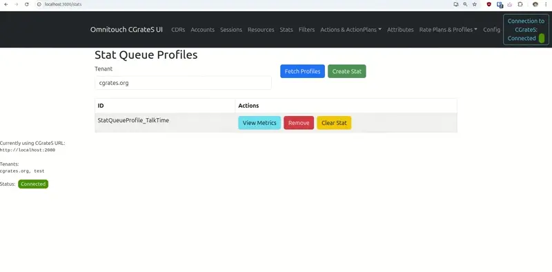
Well we’ve created a StatQueueProfile named StatQueueProfile_VoiceStats, in which we’ll store a maximum of 10000000 datapoints (this is important because to calculate an average we need to know all the previous datapoints), for a maximum of forever (Because TTL is -1, if we wanted to store for 1 hour we’d set TTL to 1h.
We’re not matching any FilterIDs, but based on what we covered on the post in FilterS, you can imagine using this to match calls from a given Account / customer, or to a specific group of destinations, or maybe from a given supplier, etc, etc.
What we do have that’s interesting is we have defined a series of metrics.
So what happens if we now generate a bunch of calls? Well, for starters as we’ve got no FilterS defined here, every call will match this StatQueueProfile, and so we’ll collect data for each.
The example code I’ve provided in the repo for this post generates a bunch of calls, and we can check the values for all our Metrics with GetQueueStringMetrics for our :
If we’ve got a TTL set, old values that have existed in the QueueProfile longer than the TTL are removed, but we can also manually clear the values by using the ResetStatQueue endpoint:
One thing to keep in mind is you can’t modify a StatQueue object via the API without resetting the values.
string_indexed_fields in the config file
Sidebar on this – By specifying the string_indexed_fields means that CGrateS will not evaluate every field against Filter rules, but instead only those defined here. This means if you’ve got an event with say 20 fields (AnswerTime, Account, Subject, Destination, RunID, SetupTime, Extra Fields, etc, etc) each of these gets evaluated against a filter, which is pretty processor intensive if your FilterS only ever look at Account and Destination, so by specifying which fields are indexed here to only the fields you use in your filters, you can boost your performance. On the flip side, you can leave this blank to evaluate all fields, but you’ll take a performance hit by doing so.
Up until this point in the series, I’ve tried to hide all the complexity of CGrateS, so people following along can see some progress and feel like they’re making it somewhere with CGrateS, but it’s time to tear off the plaster and talk about the actual concepts, about what’s under the hood, and how all the components interact, as it’ll make it much easier then for us to learn more about how to use CGrateS.
This will be the last post in the “CGrateS in Baby Steps” series (Which I started in 2022), if you’ve made it this far congratulations, all the future posts will be on specific topics and build upon the concepts we’ve covered here.
This took me a while to grasp – CGrateS is both crazy complex and beautifully simple, but getting to the stage where you can “see through the matrix” on CGrateS and see the beautiful simplicity involves a bit of understanding how everything fits together.
Once you realize once you can see the pattern, and understand the building blocks, everything else CGrateS related becomes super simple.
Agents
in CGrateS Agents are consumers of the services. That’s a super generic answer, but let’s take a closer look at what that actually means with some examples:
Diameter is a protocol that can be used for Online Charging.
CGrateS has a common interface for API calls that can perform Online Charging.
The CGrateS Diameter Agent translates between Diameter on one side, and CGrateS API calls on the other.
Likewise, if we want to speak Radius, we can use the CGrateS Radius Agent, this translates between RADIUS and the CGrateS API calls.
FreeSWITCH, Asterisk and Kamailio don’t use specific protocols like Diameter or Radius, but rather modules or plugins to connect that application to a CGrateS Agent, and they all just end up talking the same CGrateS API calls.
Lastly, there’s even an HTTP agent so you could define your own agent to talk another protocol if you wanted to use CGrateS for anything else (We’ve been playing with CAMEL based charging with CGrateS and 5GC charging).
The config for each of the CGrateS Agents happens in the cgrates.json config file (Typically in /etc/cgrates).
Because the Agents just translate everything into API calls, logic for billing a call from FreeSWITCH is the same as for Diameter, the same as for RADIUS, the same as for SIP, the same as for Asterisk.
The Agents just translate all the domain-specific stuff into the common CGrateS RPC API, which we’ve been working with up to this point.
This is key part to understand; because once you understand how to do the CGrateS part, moving from Asterisk to FreeSWITCH, to DNS, to RADIUS, to any other Agent, it’s all the same to you.
The Agents just translate domain-specific stuff (Diameter requests, CSV files, Asterisk Calls, FreeSWITCH calls, etc, etc) and act as a translator to translate these requests into CGrateS RPC API calls.
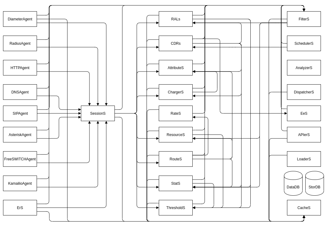
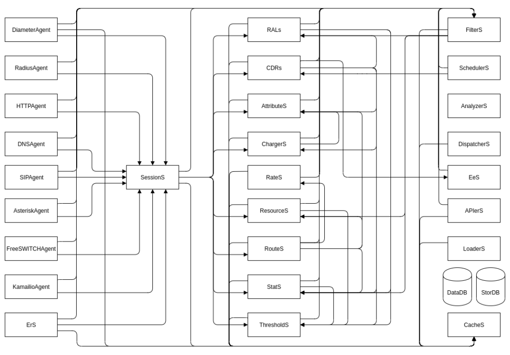
On the left side of the image below are the Agents, and on the right side, the Subsystems that do stuff with things.
Subsystems
So with these API calls, where do they go, what do they do?
Well, it’s the Subsystems that do the things.
What things?
Well, everything of use.
Each subsystem has a purpose, AttributeS transforms stuff, EeS exports CDRs, RALs applies our charging logic, CDRs writes CDRs to StorDB, etc, etc.
In each event we can set flags to denote which subsystems it should be routed to, and we can set the links between components in our cgrates.json file.
Based on the flags, we pass events between these subsystems.
Events
So our Agents create the API calls, which contain Events, which are JSON RPC calls.
They look like all the API examples we’ve played with, because that’s exactly what they are.
We can access them via the JSON RPC API, but when you start a call on Kamailio, the Kamailio Agent generates a JSON RPC API call containing an Event into CGrateS for that call on Kamailio.
When you send a DNS request, the DNS Agent translate this DNS request into a CGrateS JSON RPC API containing the event for the DNS request.
Let’s take an example, we’re going to use the ErS as it’s the simplest to demonstrate with.
So if you setup your enviroment per the tutorial above (but don’t load the CSV yet), we’ll start running some experiments…
Anatomy of an Event
We can “sniff” the events bouncing around between the Agent and the various Subsystems in real time, by using ngrep:
sudo ngrep -t -W byline port 2012 or port 2080 or port 8021 or port 2014 or port 2053 -d any
So let’ we’ve got ngrep running, we can move our CSV file in to be processed in another tab.
Plonking the CSV file into the path ERS is monitoring will mean the ErS Agent will generate a CGrateS JSON RPC “event” for each row in the file, it’ll look something like this:
Sidebar – you’re going to spend a lot of time with `ngrep`.
Alright, that event probably looks familiar, after all, it’s the same structure as the API requests we’ve made to CGrateS so far, to set rates and handle accounts.
But what we’re witnessing here isn’t us making an API request to the JSON RPC interface from a Python script, it’s the ERS Agent inside CGrateS, calling CGrateS.
The ERS Agent inside CGrateS reads the CSV file we dropped in, and based on what we had set in the ERS section of the CGrateS config file (cgrates.json), the ERS Agent create JSON RPC events and sent it to CGrateS for processing.
You may be thinking “Wow, the ERS Agent is really dumb, it just sends an API request (events)”, and you’d be right.
We could replace the ERS Agent with a Python script to read the CSV and send the same request, and we’d get the exact same outcome, but CGrateS is mostly “batteries included” so we don’t have to.
Ok, so you’ve heard me drum in the fact that Agents are pretty simple, and all they do is make JSON RPC requests for the event which are sent to CGrateS. So now what happens?
Well, the event is calling CDRsV1.ProcessEvent, so that means the Event is passed by CGRengine to the CDRs subsystem.
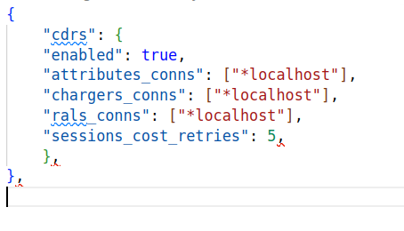
What does CDRs subsystem do with it? Well, that’s going to depend on what’s in our cgrates.json config file,
In the above example, CDRs is setup with connections to the different subsystems, AttributeS, Chargers and RALs are all the subsystems linked from here.
Having these links here does not force the Event to always route to these Subsystems, but unless we’ve got the links there, the Event won’t be able to get routed from CDRs to that subsystem if we want it to.
But we can see what’s going to happen with this request based on our CDRsV1.ProcessEvent event, it’s got Flags set to rals, so we know it wants RALs to be called.
So looking in ngrep we see our CDRsV1.ProcessExternalCDR event makes it to the CDRs module with ID 1.
The API call has flags set to *rals so the CDRs will call RALs , and inside our config the CDRs section has a link in the config (shown in the image below) to RALs (rals_conns) – if we didn’t have that link, CGrateS wouldn’t know how to connect to RALs, and the event would fail.
Note at the bottom the APIOpts section tells us this API call was made by the *cdrs subsystem and the ID is 2 (This is a different request to the original CDRsV1.ProcessExternalCDR request which had ID 1 – we can use this to match responses to requests).
Again, because our config also includes links ChargerS and RALS subsystems, we’ll see requests to (you guessed it) ChargerS (The ChargerSv1.ProcessEvent) and RALS (Responder.GetCost).
# T 2024/12/22 09:09:47.465711 127.0.0.1:2012 -> 127.0.0.1:50456 [AP] #414 {"id":4,"result":{"Category":"call","Tenant":"cgrates.org","Subject":"61812341234","Account":"61412341234","Destination":"61812341234","ToR":"*voice","Cost":14,"Timespans":[{"TimeStart":"2024-01-01T01:00:00+11:00","TimeEnd":"2024-01-01T01:01:00+11:00","Cost":14,"RateInterval":{"Timing":{"ID":"*any","Years":[],"Months":[],"MonthDays":[],"WeekDays":[],"StartTime":"00:00:00","EndTime":""},"Rating":{"ConnectFee":0,"RoundingMethod":"*up","RoundingDecimals":4,"MaxCost":0,"MaxCostStrategy":"","Rates":[{"GroupIntervalStart":0,"Value":14,"RateIncrement":60000000000,"RateUnit":60000000000}]},"Weight":10},"DurationIndex":60000000000,"Increments":[{"Duration":0,"Cost":0,"BalanceInfo":{"Unit":null,"Monetary":null,"AccountID":""},"CompressFactor":1},{"Duration":60000000000,"Cost":14,"BalanceInfo":{"Unit":null,"Monetary":null,"AccountID":""},"CompressFactor":1}],"RoundIncrement":null,"MatchedSubject":"*out:cgrates.org:call:*any","MatchedPrefix":"618","MatchedDestId":"Dest_AU_Fixed","RatingPlanId":"RatingPlan_VoiceCalls","CompressFactor":1}],"RatedUsage":60000000000,"AccountSummary":null},"error":null}
What we’re seeing is the CDRs module, calling RALs, to get the cost information for this event.
Finally the CDRsV1.ProcessEvent that was initially sent by ErS gets a result (we can find the result to the request as it’ll have the same id parameter)
So that’s it, that’s the secret sauce – CGrateS is just a bunch of little APIs we combo together to create something great.
Recap
Agents translate data sources into API calls.
Each little API belongs to a Subsystem, like ChargerS, AttributeS or RALs, and we can chain them together in our config file or through the flags in the API request.
Once you’ve got your head wrapped around this, everything in CGrateS becomes way easier.
From now on I’ll pivot to talking about specific modules, and how we use them, starting with AttributeS (which I wrote last year while still drafting this), and diving into how to use each module in more detail.
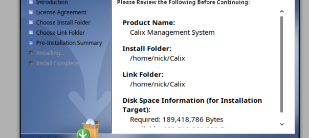
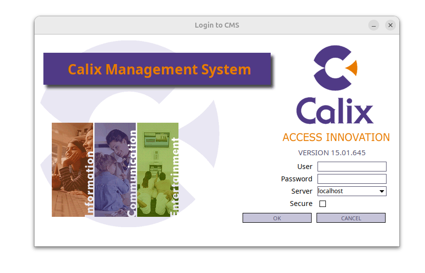
Ah, another post in my “how to make software work that was made with Java in the 1990s” post, except Calix last updated this software in 2022 – make of that what you will…
This time is Calix Management System (CMS), the Java app for managing equipment in exchanges / COs from Calix.
I generally do this with Python or via the Swagger UI for the Web UI, but here’s how we can create a fixed-line IMS subscriber in PyHSS, so we can register it with a softphone, without using EAP-AKA.
Firstly we create the AuC object for this password combo.
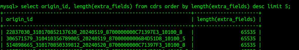
I started seeing this error the other day when running CDRsv1.GetCDRs on the CGrateS API:
SERVER_ERROR: unexpected end of JSON input
It seemed related to certain CDRs in the cdrs table of StoreDB.
After some digging, I found the stupid simple problem:
I’d written too much data to extra_fields, leading MySQL to cut off the data mid way through, meaning it couldn’t be reconstructed as JSON by CGrateS again.
Like the rounding issue I had, this wasn’t an issue with CGrateS but with MySQL.
Quick fix:
sudo mysql cgrates -e "ALTER TABLE cdrs MODIFY extra_fields LONGTEXT;"
And new fields can exceed this length without being cut off.
Like a lot of companies, we’re moving away from VMware, and in our case, shifting to Proxmox.
But that doesn’t mean we can get entirely away from VMware, but more that it’s not our hypervisor of choice anymore, and this means shifting our dev environments and lab off VMware to Proxmox first.
So today I sat down to try and shift everything to Proxmox, while keeping the VMware based VMs accessible until they can slowly die of bitrot.
A sane person would probably utilize Proxmox’s fancy new tool for migrating VMs from VMware to Proxmox, and it’s great, but in our case at least, it required logging into each VM and remapping NICs, etc, which is tricky on boxes I don’t have access to – Plus we need to keep some VMware capability for testing / labbing stuff up.
So I decided into install Proxmox onto the bare metal servers, and then create a VMware virtual machine inside the Proxmox stack, to host a VMware ESXi instance.
I started off inside VMware (Before installing any Proxmox) by moving all the VMs onto a single physical disk, which I then removed from the server, so as to not accidentally format the one disk I didn’t want to format.
Next I nuked the server and setup the new stack with Proxmox, which is a doddle, and not something I’ll cover.
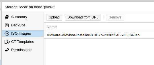
Then I loaded a VMware ISO into Proxmox and started setting up the VM.
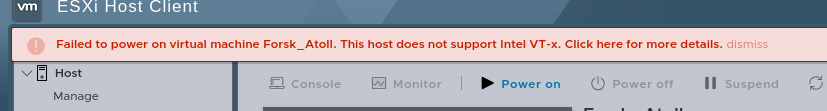
Now, nested virtualization is a real pain in the behind.
VMware doesn’t like not being run on bare metal, and it took me a good long amount of time to find the hardware config that I could setup in Proxmox that VMware would accept.
Create the VM in the Web UI; I found using a SATA drive worked while SCSI failed, so create a SATA based LVM image to use, and mount the datastore ISO.
Then edit /etc/pve/qemu-server/your_id.conf and replace the netX, args, boot and ostype to match the below:
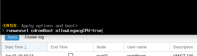
Now you can go and start the VM, but once you’ve got the VMware splash screen, you’ll need to press Shift + O to enter the boot options.
At the runweasle cdromBoot after it add allowLegacyCPU=true– This will allow ESXi to use our (virtual) CPU.
Next up you’ll install VMware ESXi just like you’ve probably done 100 times before (is this the last time?), and once it’s done installing, power off, we’ll have to make few changes to the VM definition file.
Then after install we need to change the boot order, by updating:
boot: order=sata0
And unmount the ISO:
ide2: none,media=cdrom
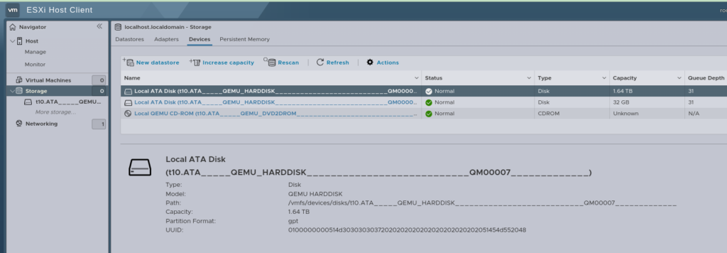
Now remember how I’d pulled the hard disk containing all the VMware VMs out so I couldn’t break it? Well, don’t drop that, because now we’re going to map that physical drive into the VM for VMware, so I can boot all those VMs.
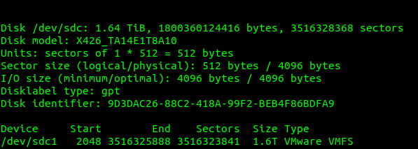
I plugged in the drive and I used this to find the drive I’d just inserted:
fdisk -l
Which showed the drive I’d just added last, with it’s VMware file system.
So next we need to map this through the VM we just created inside Proxmox, so VMware inside Proxmox can access the VMware file system on the disk filled with all our old VMware VMs.
VM. VM. VM. The word has lost all meaning to me at this stage.
We can see the mount point of our physical disk; in our case is /dev/sdc so that’s what we’ll pass through to the VM.
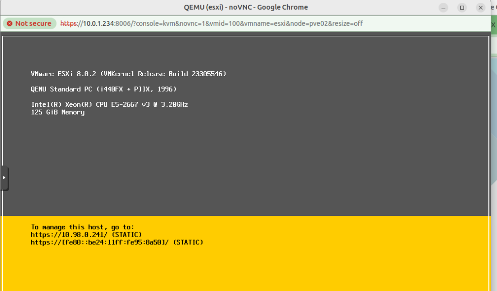
And now, if everything has gone well, after logging into the Web UI, you’ll see this:
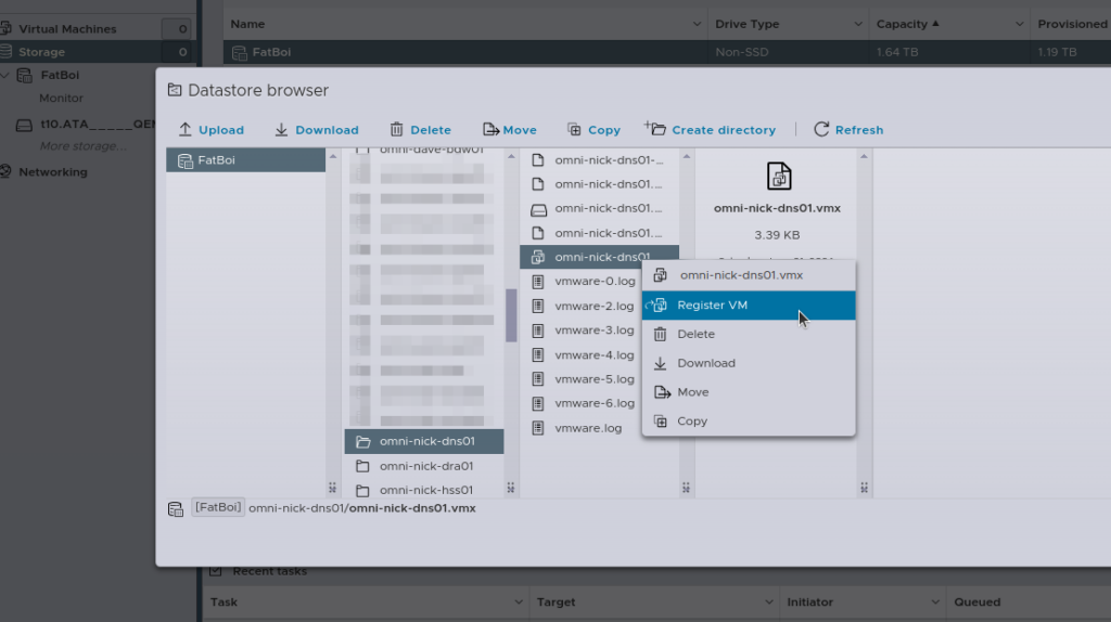
Then the last step is going to be re-registering all the VMs, you can do this by hand, by selecting the .vmx file and adding it.
Alternately, if you’re lazy like me, I wrote a little script to do the same thing:
[root@localhost:~] cat load_vms3.sh


#!/bin/bash

# Datastore name
DATASTORE="FatBoi/"

# Log file to store the output
LOG_FILE="/var/log/register_vms.log"

# Clear the log file
> $LOG_FILE

echo "Starting VM registration process on datastore: $DATASTORE" | tee -a $LOG_FILE

# Check if datastore directory exists
if [ ! -d "/vmfs/volumes/$DATASTORE" ]; then
    echo "Datastore $DATASTORE does not exist!" | tee -a $LOG_FILE
    exit 1
fi

# Find all .vmx files in the datastore and register them
find /vmfs/volumes/$DATASTORE -type f -name "*.vmx" | while read VMX_PATH; do
    echo "Registering VM: $VMX_PATH" | tee -a $LOG_FILE
    vim-cmd solo/registervm "$VMX_PATH" | tee -a $LOG_FILE
done

echo "VM registration process completed." | tee -a $LOG_FILE

[root@localhost:~] sh load_vms3.sh
Now with all your VMs loaded, you should almost be ready to roll and power them all back on.
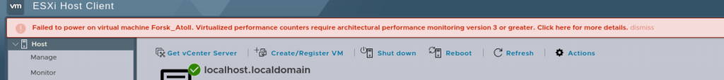
But before we reboot the Hypervisor (Proxmox) we’ll have to reboot the VMware hypervisor too, because here’s something else to make you punch the screen:
Luckily we can fix this one globaly.
SSH into the VMware box, edit /etc/vmware/config.xml file and add:
vhv.enable = "FALSE"
Which will disable the performance counters.
Now power off the VMware VM, and reboot the Proxmox hypervisor, when it powers on again, Proxmox will allow nested virtualization, and when you power back on the VMware VM, you’ll have performance counters disabled, and then, you will be done.
Yeah, not a great use of my Saturday, but here we are…