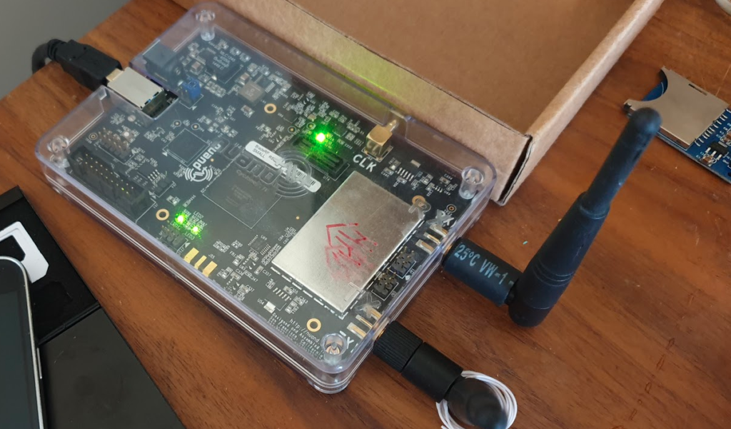
The team at Software Radio Systems in Ireland have been working on an open source LTE stack for some time, to be used with software defined radio (SDR) hardware like the USRP, BladeRF and LimeSDR.
They’ve released SRSUE and SRSENB their open source EUTRAN UE and eNodeB, which allow your SDR hardware to function as a LTE UE and connect to a commercial eNB like a standard UE while getting all the juicy logs and debug info, or as a LTE eNB and have commercial UEs connect to a network you’re running, all on COTS hardware.
The eNB supports S1AP to connect to a 3GPP compliant EPC, like Open5Gs, but also comes bundled with a barebones EPC for testing.
The UE allows you to do performance testing and gather packet captures on the MAC & PHY layers, something you can’t do on a commericial UE. It also supports software-USIMs (IMSI / K / OP variables stored in a text file) or physical USIMs using a card reader.
I’ve got a draw full of SDR hardware, from the first RTL-SDR dongle I got years ago, to a few HackRFs, a LimeSDR up to the BladeRF x40.
Really cool software to have a play with, I’ve been using SRSUE to get a better understanding of the lower layers of the Uu interface.
Installation
After mucking around trying to satisfy all the dependencies from source I found everything I needed could be found in Debian packages from the repos of the maintainers.
To begin with we need to install the BladeRF drivers and SopySDR modules to abstract it to UHD:
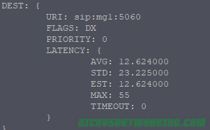
One question that’s not as obvious as it perhaps should be is the different states shown with kamcmd dispatcher.list command;
So what do the flags for state mean?
The first letter in the flag means is the current state, Active (A), Inactive (I) or Disabled (D).
The second letter in the flag means monitor status, Probing (P) meaning actively checked with SIP Options pings, or Not Set (X) denoting the device isn’t actively checked with SIP Options pings.
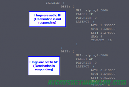
AP – Actively Probing – SIP OPTIONS are getting a response, routing to this destination is possible, and it’s “Up” for all intents and purposes.
IP – Inactively Probing – Destination is not meeting the threshold of SIP OPTIONS request responses it needs to be considered active. The destination is either down or not responding to all SIP OPTIONS pings. Often this is due to needing X number of positive responses before considering the destination as “Up”.
DX – Disabled & Not Probing – This device is disabled, no SIP OPTIONS are sent.
AX – Active & Not Probing– No SIP OPTIONS are sent to check state, but is is effectively “Up” even though the remote end may not be reachable.
In the third part of the Kamailio 101 series I briefly touched upon pseudovariables, but let’s look into what exactly they are and how we can manipulate them to change headers.
The term “pseudo-variable” is used for special tokens that can be given as parameters to different script functions and they will be replaced with a value before the execution of the function.
You’ve probably seen in any number of the previous Kamailio Bytes posts me use pseudovariables, often in xlog or in if statements, they’re generally short strings prefixed with a $ sign like $fU, $tU, $ua, etc.
When Kamailio gets a SIP message it explodes it into a pile of variables, getting the To URI and putting it into a psudovariable called $tU, etc.
We can update the value of say $tU and then forward the SIP message on, but the To URI will now use our updated value.
When it comes to rewriting caller ID, changing domains, manipulating specific headers etc, pseudovariables is where it mostly happens.
Kamailio allows us to read these variables and for most of them rewrite them – But there’s a catch. We can mess with the headers which could result in our traffic being considered invalid by the next SIP proxy / device in the chain, or we could mess with the routing headers like Route, Via, etc, and find that our responses never get where they need to go.
So be careful! Headers exist for a reason, some are informational for end users, others are functional so other SIP proxies and UACs can know what’s going on.
Rewriting SIP From Username Header (Caller ID)
When Kamailio’s SIP parser receives a SIP request/response it decodes the vast majority of the SIP headers into a variety of pseudovariables, we can then reference these variables we can then reference from our routing logic.
Let’s pause here and go back to the Stateless SIP Proxy Example, as we’ll build directly on that.
Follow the instructions in that post to get your stateless SIP proxy up and running, and we’ll make this simple change:
####### Routing Logic ########


/* Main SIP request routing logic
 * - processing of any incoming SIP request starts with this route
 * - note: this is the same as route { ... } */
request_route {

        xlog("Received $rm to $ru - Forwarding");
        $fU = "Nick Blog Example";   #Set From Username to this value
        #Forward to new IP
        forward("192.168.1.110");

}
Now when our traffic is proxied the From Username will show “Nick Blog Example” instead of what it previously showed.
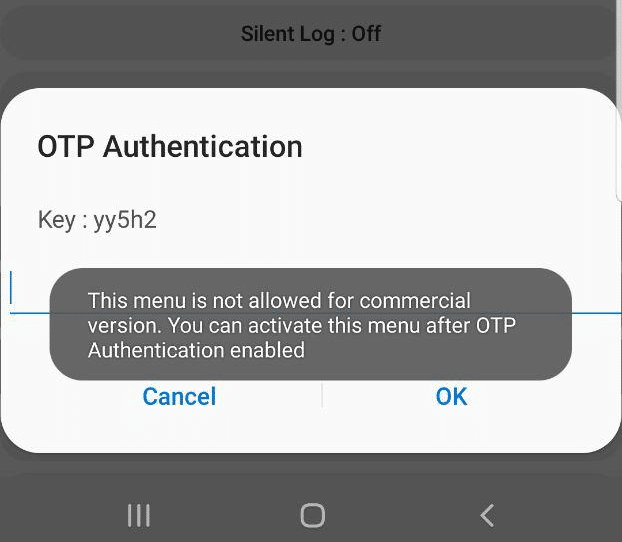
While poking around the development and debugging features on Samsung handsets I found the ability to run IMS Debugging directly from the handset.
Alas, the option is only available in the commercial version, it’s just there for carriers, and requires a One Time Password to unlock.
When tapping on the option a challenge is generated with a key.
Interestingly I noticed that the key changes each time and can reject you even in aeroplane mode, suggesting the authentication happens client side.
This left me thinking – If the authentication happens client side, then the App has to know what the valid password for the key shown is…
Some research revealed you can pull APKs off an Android phone, so I downloaded a utility called “APK Extractor” from the Play store, and used it to extract the Samsung Sysdump utility.
So now I was armed with the APK on my local machine, the next step was to see if I could decompile the APK back into source code.
Some Googling found me an online APK decompiler, which I fed the compiled APK file and got back the source code.
I did some poking around inside the source code, and then I found an interesting directory:
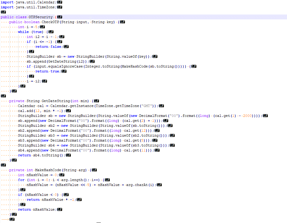
Here’s a screenshot of the vanilla code that came out of the app.
I’m not a Java expert, but even I could see the “CheckOTP” function and understand that that’s what validates the One Time Passwords.
The while loop threw me a little – until I read through the rest of the code; the “key” in the popup box is actually a text string representing the current UNIX timestamp down to the minute level. The correct password is an operation done on the “key”, however the CheckOTP function doesn’t know the challenge key, but has the current time, so generates a challenge key for each timestamp back a few minutes and a few minutes into the future.
I modified the code slightly to allow me to enter the presented “key” and get the correct password back. It’s worth noting you need to act quickly, enter the “key” and enter the response within a minute or so.
In the end I’ve posted the code on an online Java compiler,
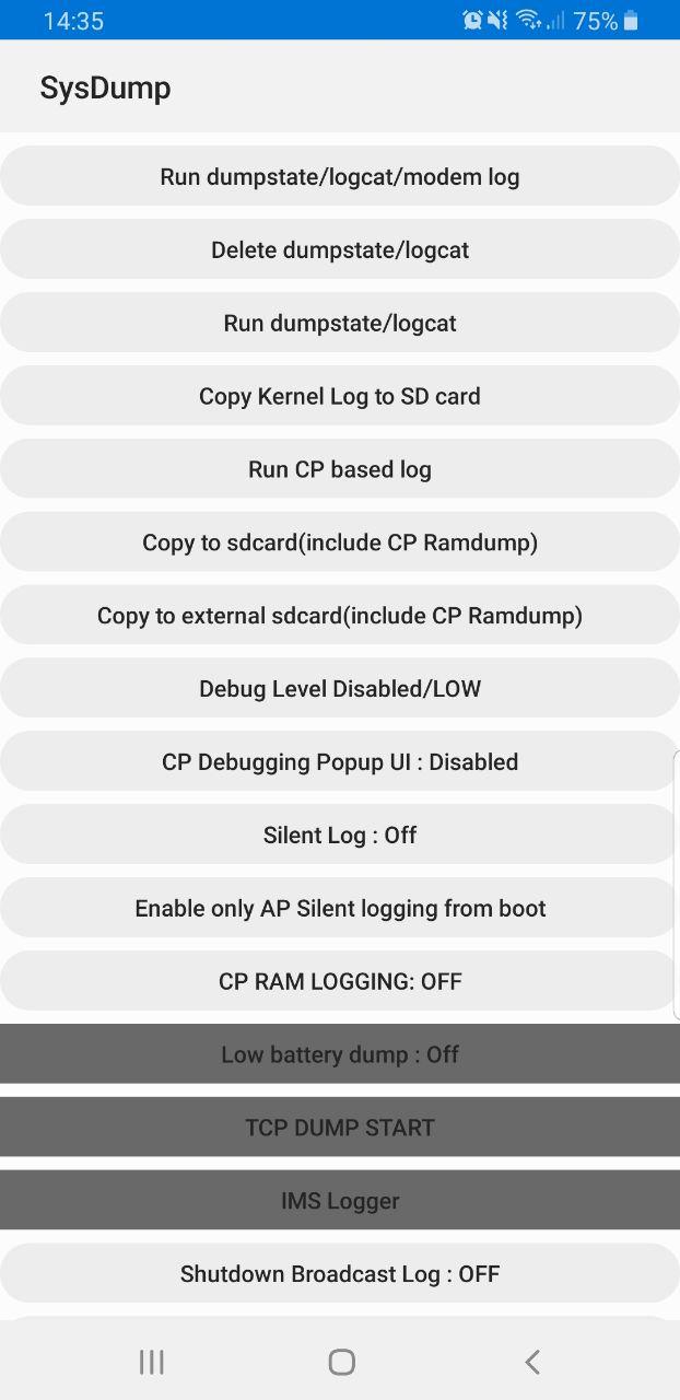
Samsung handsets have a feature built in to allow debugging from the handset, called Sysdump.
Entering *#9900# from the Dialing Screen will bring up the Sysdump App, from here you can dump logs from the device, and run a variety of debugging procedures.
But for private LTE operators, the two most interesting options are by far the TCPDUMP START option and IMS Logger, but both are grayed out.
Tapping on them asks for a one-time password and has a challenge key.
These options are not available in the commercial version of the OS and need to be unlocked with a one time key generated by a tool Samsung for unlocking engineering firmware on handsets.
Luckily this authentication happens client side, which means we can work out the password it’s expecting.
Once you’ve entered the code and successfully unlocked the IMS Debugging tool there’s a few really cool features in the hamburger menu in the top right.
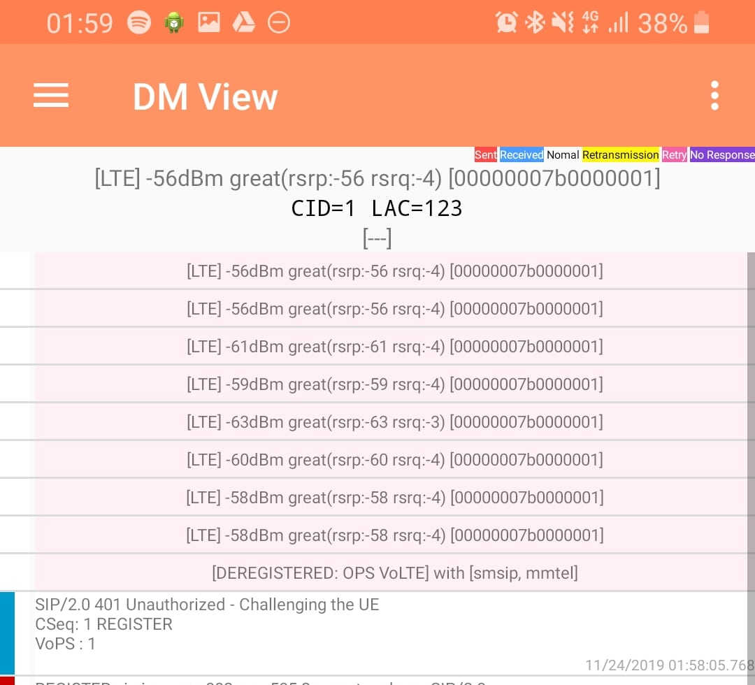
DM View
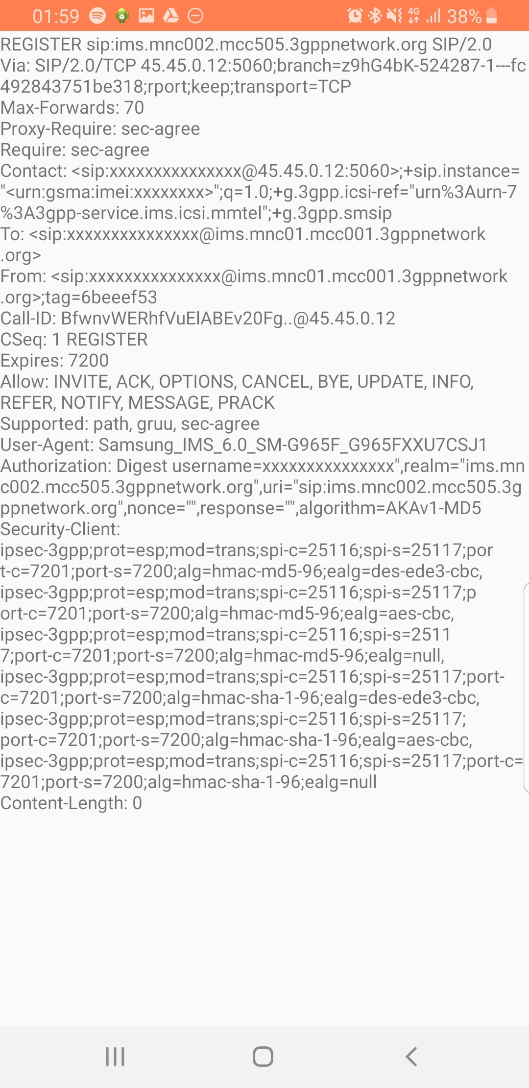
This shows the SIP / IMS Messaging and the current signal strength parameters (used to determine which RAN type to use (Ie falling back from VoLTE to UMTS / Circuit Switched when the LTE signal strength drops).
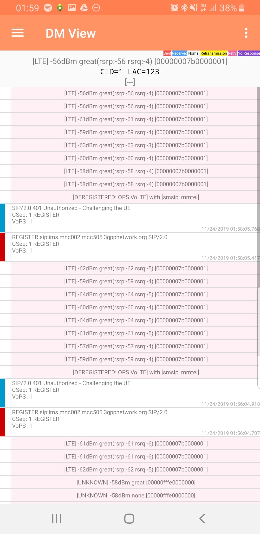
Tapping on the SIP messages expands them and allows you to see the contents of the SIP messages.
Viewing SIP Messaging directly from the handset
Interesting the actual nitty-gritty parameters in the SIP headers are missing, replaced with X for anything “private” or identifiable.
Luckily all this info can be found in the Pcap.
The DM View is great for getting a quick look at what’s going on, on the mobile device itself, without needing a PC.
Logging
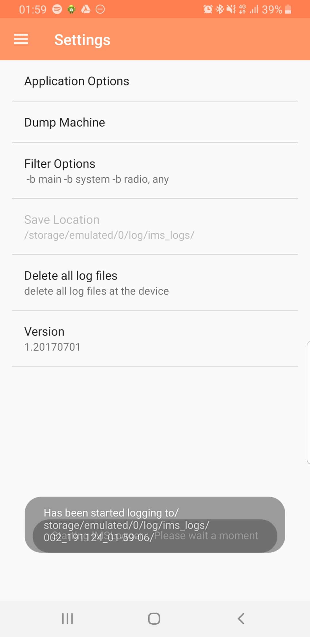
The real power comes in the logging functions,
There’s a lot of logging options, including screen recording, TCPdump (as in Packet Captures) and Syslog logging.
From the hamburger menu we can select the logging parameters we want to change.
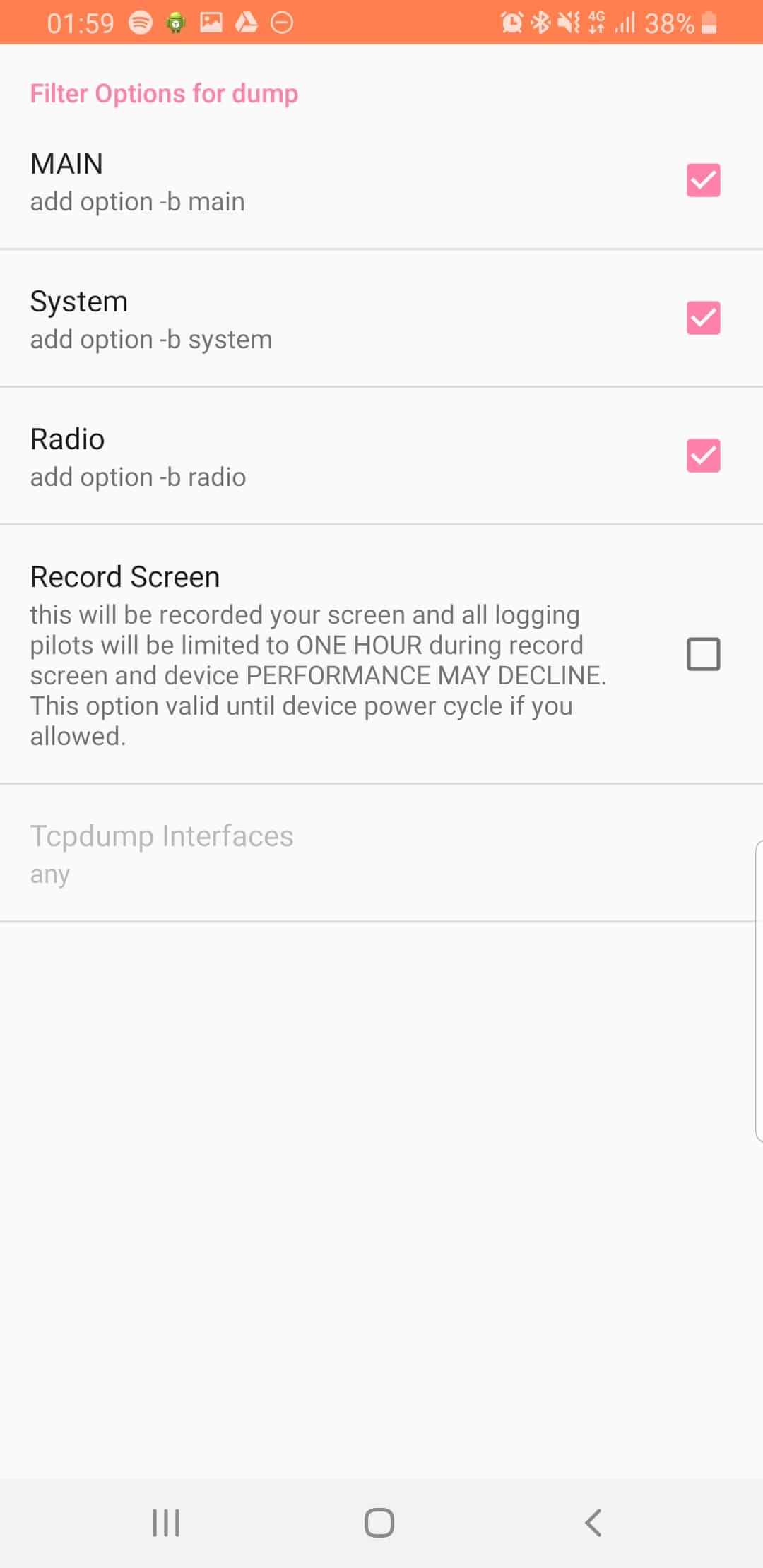
From the Filter Options menu we can set what info we’re going to log,
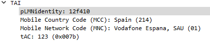
The PLMN Identifier is used to identify the radio networks in use, it’s made up of the MCC – Mobile Country Code and MNC – Mobile Network Code.
But sadly it’s not as simple as just concatenating MCC and MNC like in the IMSI, there’s a bit more to it.
In the example above the Tracking Area Identity includes the PLMN Identity, and Wireshark has been kind enough to split it out into MCC and MNC, but how does it get that from the value 12f410?
This one took me longer to work out than I’d like to admit, and saw me looking through the GSM spec, but here goes:
PLMN Contents: Mobile Country Code (MCC) followed by the Mobile Network Code (MNC). Coding: according to TS GSM 04.08 [14].
If storage for fewer than the maximum possible number n is required, the excess bytes shall be set to ‘FF’. For instance, using 246 for the MCC and 81 for the MNC and if this is the first and only PLMN, the contents reads as follows: Bytes 1-3: ’42’ ‘F6′ ’18’ Bytes 4-6: ‘FF’ ‘FF’ ‘FF’ etc.
TS GSM 04.08 [14].
Making sense to you now? Me neither.
Here’s the Python code I wrote to encode MCC and MNCs to PLMN Identifiers and to decode PLMN into MCC and MNC, and then we’ll talk about what’s happening:
In the above example I take MCC 505 (Australia) and MCC 93 and generate the PLMN ID 05f539.
The first step in decoding is to take the first two bits (in our case 05 and reverse them – 50, then we take the third and fourth bits (f5) and reverse them too, and strip the letter f, now we have just 5. We join that with what we had earlier and there’s our MCC – 505.
Next we get our MNC, for this we take bytes 5 & 6 (39) and reverse them, and there’s our MNC – 93.
Together we’ve got MCC 505 and MNC 93.
The one answer I’m still looking for; why not just encode 50593? What is gained by encoding it as 05f539?
After a few quiet months I’m excited to say I’ve pushed through some improvements recently to PyHSS and it’s growing into a more usable HSS platform.
MongoDB Backend
This has a few obvious advantages – More salable, etc, but also opens up the ability to customize more of the subscriber parameters, like GBR bearers, etc, that simple flat text files just wouldn’t support, as well as the obvious issues with threading and writing to and from text files at scale.
Knock knock.
Race condition.
Who’s there?
— Threading Joke.
For now I’m using the Open5GS MongoDB schema, so the Open5Gs web UI can be used for administering the system and adding subscribers.
The CSV / text file backend is still there and still works, the MongoDB backend is only used if you enable it in the YAML file.
The documentation for setting this up is in the readme.
SQN Resync
If you’re working across multiple different HSS’ or perhaps messing with some crypto stuff on your USIM, there’s a chance you’ll get the SQN (The Sequence Number) on the USIM out of sync with what’s on the HSS.
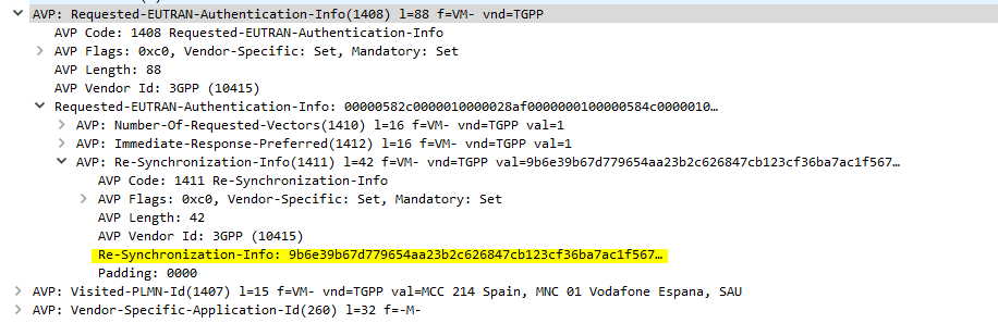
This manifests itself as an Update Location Request being sent from the UE in response to an Authentication Information Answer and coming back with a Re-Syncronization-Info AVP in the Authentication Info AVP. I’ll talk more about how this works in another post, but in short PyHSS now looks at this value and uses it combined with the original RAND value sent in the Authentication Information Answer, to find the correct SQN value and update whichever database backend you’re using accordingly, and then send another Authentication Information Answer with authentication vectors with the correct SQN.
SQN Resync is something that’s really cryptographically difficult to implement / confusing, hence this taking so long.
What’s next? – IMS / Multimedia Auth
The next feature that’s coming soon is the Multimedia Authentication Request / Answer to allow CSCFs to query for IMS Registration and manage the Cx and Dx interfaces.
Code for this is already in place but failing some tests, not sure if that’s to do with the MAA response or something on my CSCFs,
The Australian Government publishes elevation data online that’s freely available for anyone to use. There’s a catch – If you’re using Forsk Atoll, it won’t import without a fair bit of monkeying around with the data…
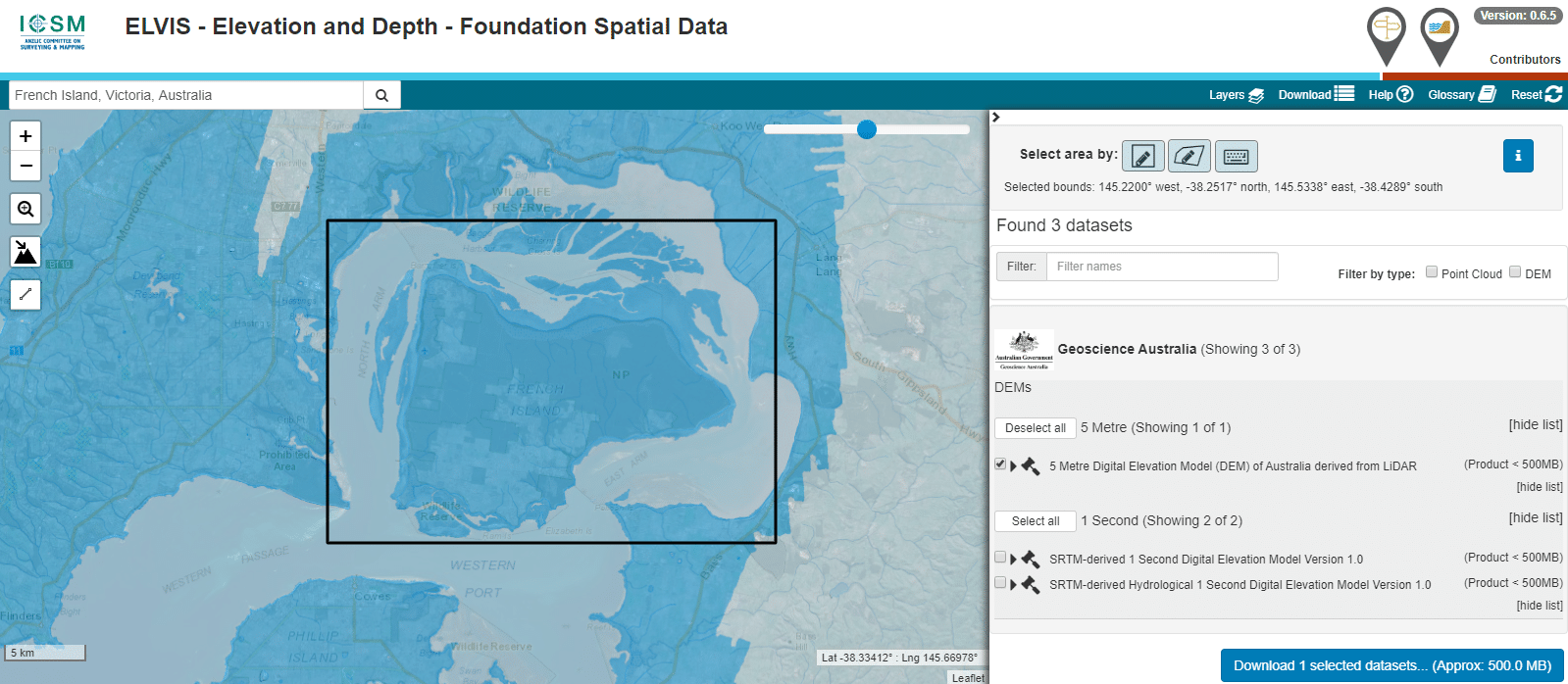
You draw around the area you want to download, enter your email address and you’re linked to a download of the dataset you’ve selected.
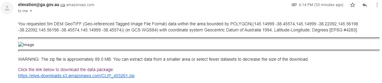
So now we download the data from the link, unzip it and we’re provided with a .tiff image with the elevation data in the pixel colour and geocoded with the positional information.
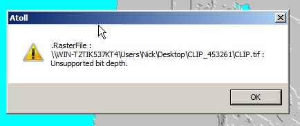
Problem is, this won’t import into Atoll – Unsupported depth.
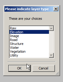
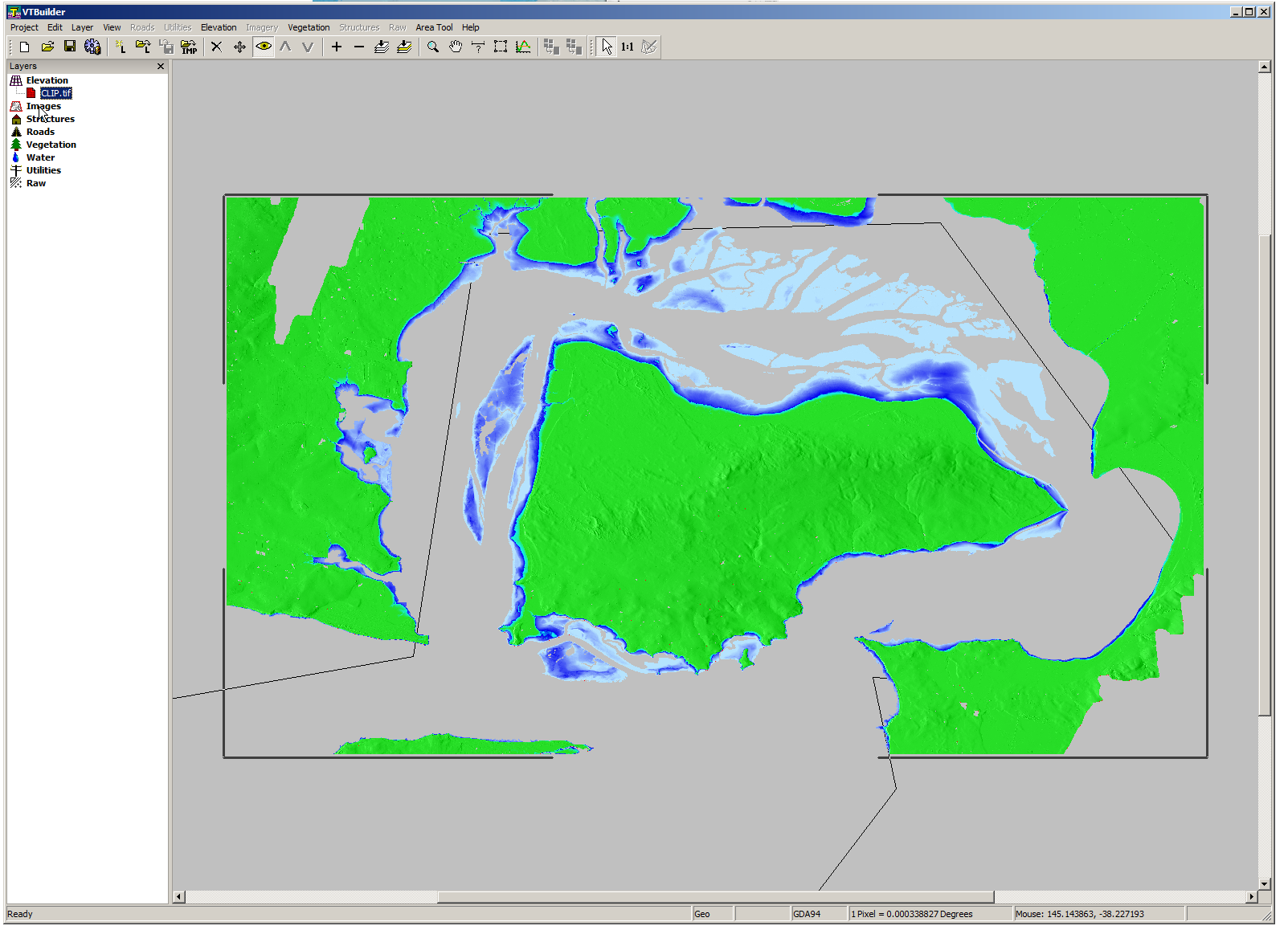
I fired it up, and imported the elevation tiff file we’d downloaded.
Selected “Elevation” waited a few seconds and presto!
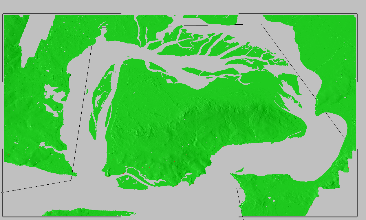
We can export from here in the PNG 16 bit grayscale format Atoll takes, but there’s a catch, negative elevation values and blank data will show up as giant spikes which will totally mess with your propagation modeling.
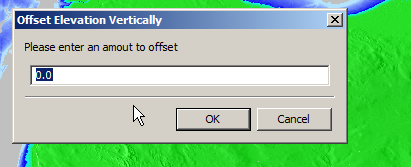
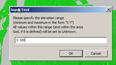
So I found an option to remove elevation data from a set range, but it won’t deal with negative values…
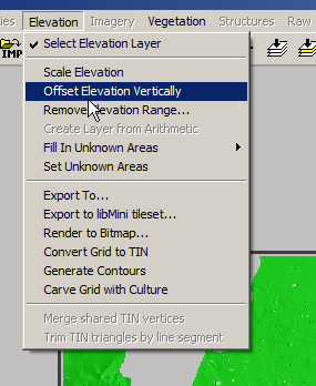
So I found another option in the elevation menu to offset elevation vertically, I added 100 ft (It’s all in ft for some reason) to everything which meant my elevation data that was previously negative was now just under 100.
So if an area was -1ft before it was now 99ft.
Now I was able to use the remove range for anything from 0 100 ft (previously sea level)
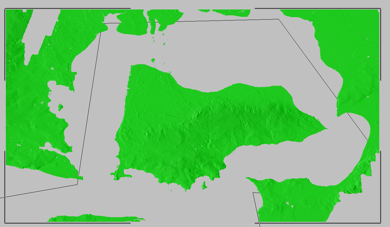
Now my map only shows data above sea level
Now I offset the elevation vertically again and remove 100ft so we get back to real values
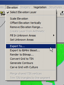
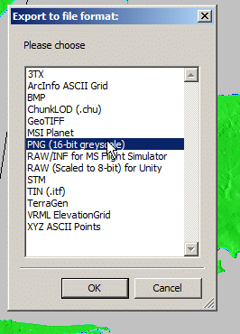
Now I was able to export the elevation data from the Elevation -> Export to menu
Atoll seems to like PNG 16 bit greyscale so that’s what we’ll feed it.
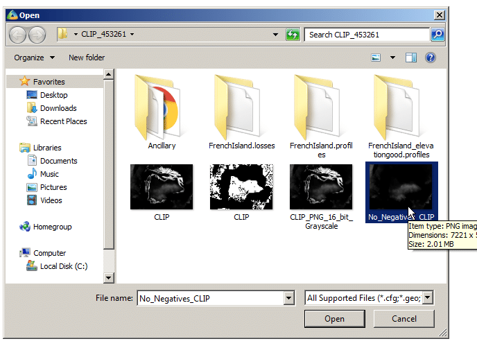
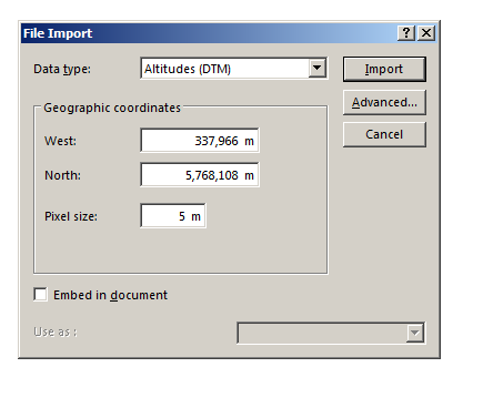
In Atoll we’ll select File -> Import and open the PNG we just generated.
Data type will be Altitude, Pixel size is 5m (as denoted in email / dataset metadata).
Next question is offset, which took me a while to work out…
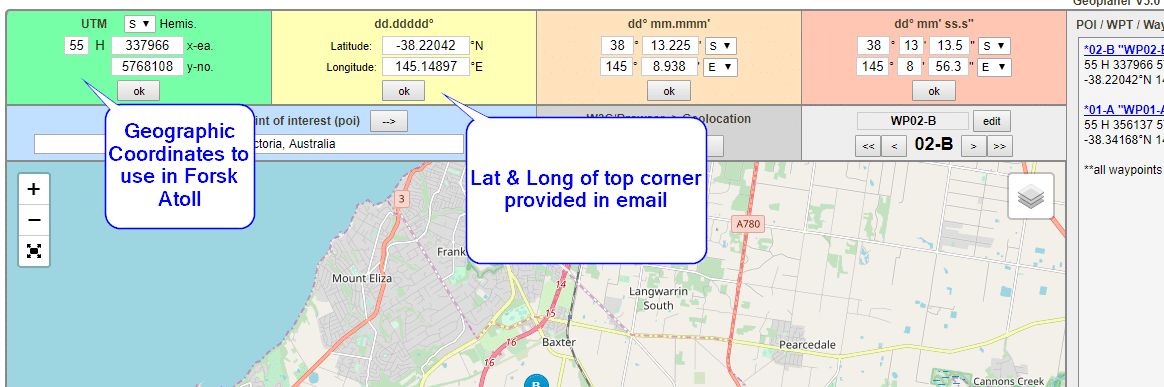
The email has the Lat & Long but Atoll deals in WGS co-ordinates,
Luckily the GeoPlanner website allows you to enter the lat & long of the top corner and get the equivalent West and North values for the UTM dataum.
Enter these values as your coordinates and you’re sorted.
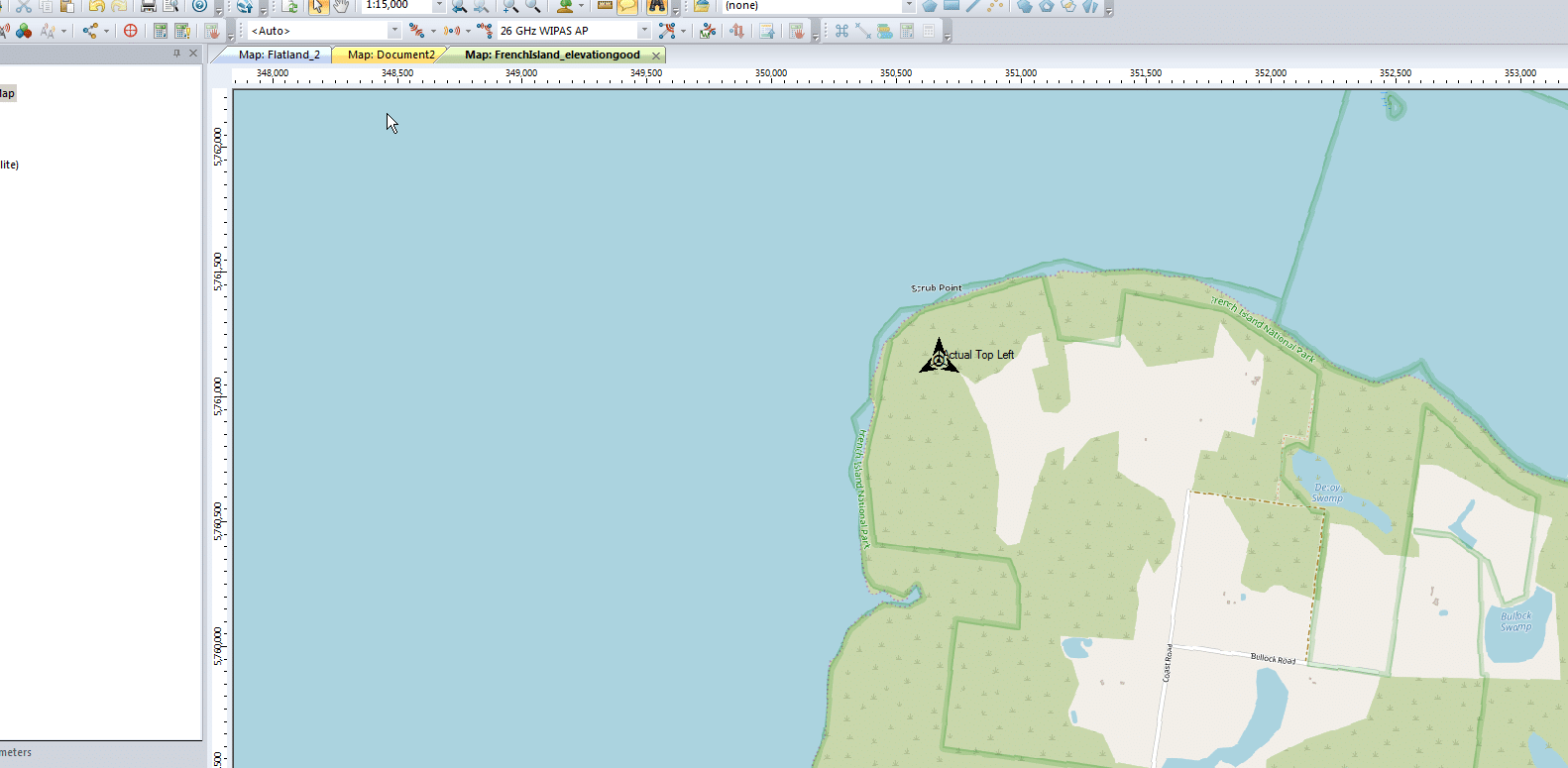
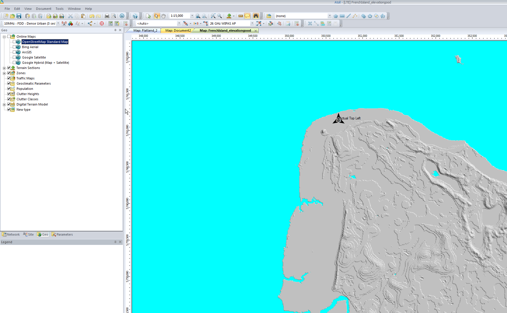
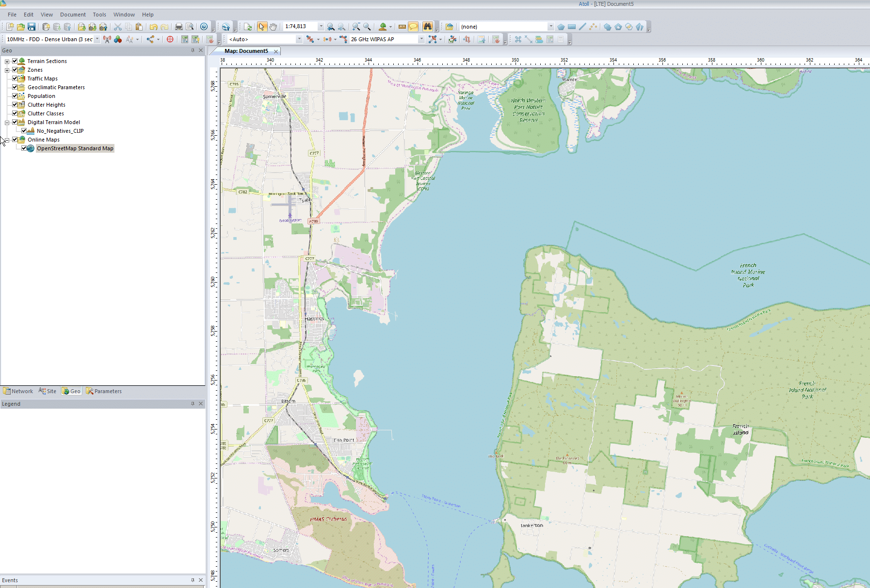
I can even able a Map layer and confirm it lines up:
Note: NextEPC the Open Source project rebranded as Open5Gs in 2019 due to a naming issue. The remaining software called NextEPC is a branch of an old version of Open5Gs. This post was written before the rebranding.
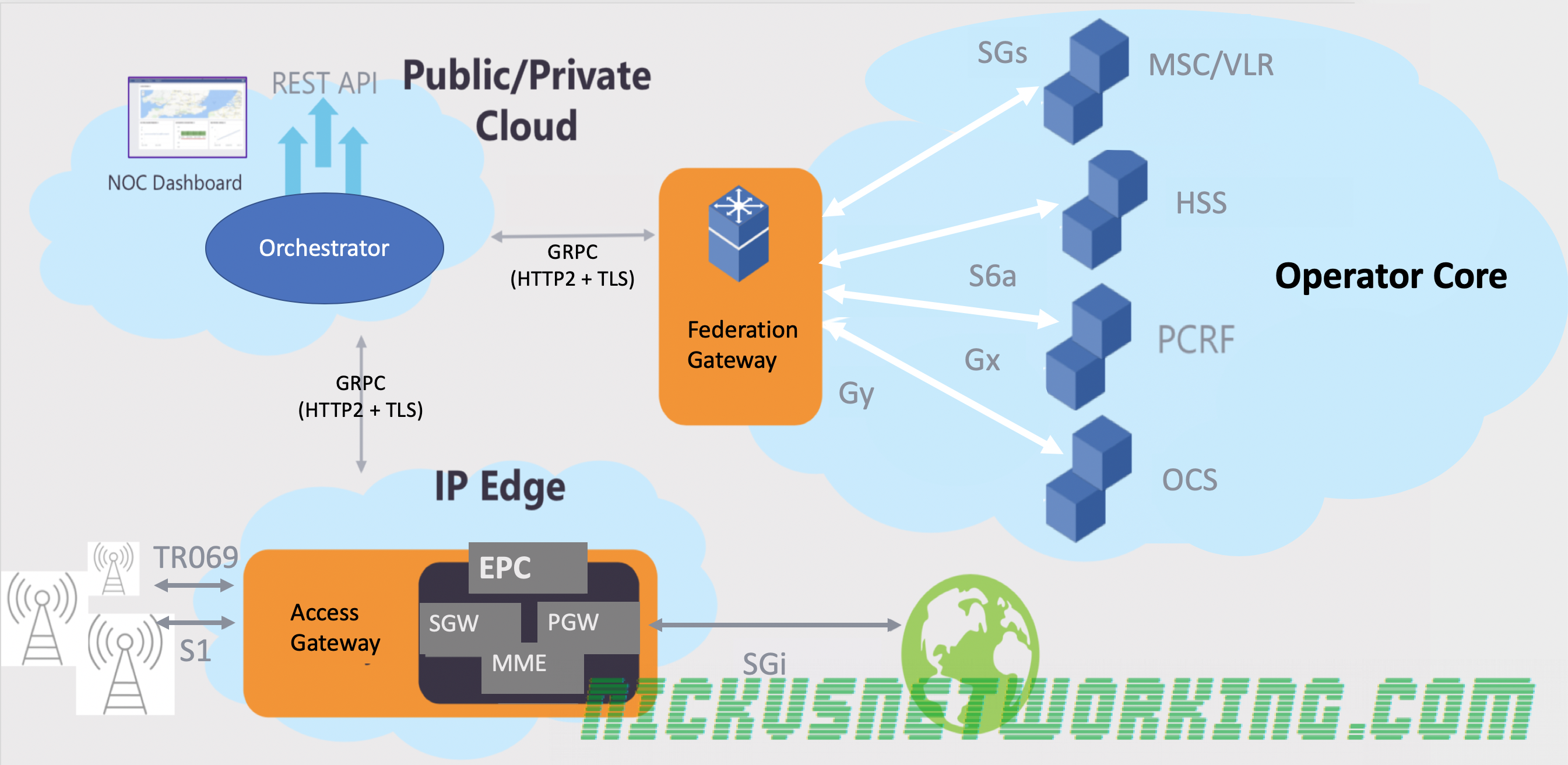
In a production network network elements would typically not all be on the same machine, as is the default example that ships with NextEPC.
NextEPC is designed to be standards compliant, so in theory you can connect any core network element (MME, PGW, SGW, PCRF, HSS) from NextEPC or any other vendor to form a functioning network, so long as they are 3GPP compliant.
To demonstrate this we will cover isolating each network element onto it’s on machine and connect each network element to the other. For some interfaces specifying multiple interfaces is supported to allow connection to multiple
In these examples we’ll be connecting NextEPC elements together, but it could just as easily be EPC elements from a different vendor in the place of any NextEPC network element.
Service
IP
Identity
P-GW
10.0.1.121
pgw.localdomain
S-GW
10.0.1.122
PCRF
10.0.1.123
pcrf.localdomain
MME
10.0.1.124
mme.localdomain
HSS
10.0.1.118
hss.localdomain
External P-GW
In it’s simplest from the P-GW has 3 interfaces:
S5 – Connection to home network S-GW (GTP-C)
Gx – Connection to PCRF (Diameter)
Sgi – Connection to external network (Generally the Internet via standard TCP/IP)
S5 Interface Configuration
Edit /etc/nextepc/pgw.confand change the address to IP of the server running the P-GW for the listener on GTP-C and GTP-U interfaces.
If you are using NextEPC’s HSS you may need to enable MongoDB access from the PCRF. This is done by editing ‘‘/etc/mongodb.conf’’ and changing the bind IP to: bind_ip = 0.0.0.0
Restart MongoDB for changes to take effect.
$ /etc/init.d/mongodb restart
External MME
In it’s simplest form the MME has 3 interfaces:
S1AP – Connections from eNodeBs
S6a – Connection to HSS (Diameter)
S11 – Connection to S-GW (GTP-C)
S11 Interface Configuration
Edit /etc/nextepc/mme.conf, filling the IP address of the S-GW and P-GW servers.
As anyone who’s setup a private LTE network can generally attest, APNs can be a real headache.
SIM/USIM cards, don’t store any APN details. In this past you may remember having to plug all these settings into your new phone when you upgraded so you could get online again.
Today when you insert a USIM belonging to a commercial operator, you generally don’t need to put APN settings in, this is because Android OS has its own index of APNs. When the USIM is inserted into the baseband module, the handset’s OS looks at the MCC & MNC in the IMSI and gets the APN settings automatically from Android’s database of APN details.
There is an option for the network to send the connectivity details to the UE in a special type of SMS, but we won’t go into that.
All this info is stored on the Android OS in apns-full-conf.xml which for non-rooted (stock) devices is not editable.
This file can override the user’s APN configuration, which can lead to some really confusing times as your EPC rejects the connection due to an unrecognized APN which is not what you have configured on the UE’s operating system, but it instead uses APN details from it’s database.
The only way around this is to change the apns-full-conf.xml file, either by modifying it per handset or submitting a push request to Android Open Source with your updated settings.
(I’ve only tried the former with rooted devices)
The XML file itself is fairly self explanatory, taking the MCC and MNC and the APN details for your network:
Once you’ve added yours to the file, inserting the USIM, rebooting the handset or restarting the carrier app is all that’s required for it to be re-read and auto provision APN settings from the XML file.
If you’re planning on using this in production you probably want to automate the pulling of this data on a regular basis and keep it in a different directory.
I’ve made a very simple example Kamailio config that shows off some of the features of GeoIP2’s logic and what can be shown, so let’s look at the basics of the module:
if(geoip2_match("$si", "src")){
                xlog("Packet received from IP $si");
                xlog("Country is: $gip2(src=>cc)\n");
}
If we put this at the top of our request_route block every time we recieve a new request we can see the country from which the packet came from.
Let’s take a look at the output of syslog (with my IP removed):
#> tail -f /var/log/syslog
ERROR: <script>: Packet received from IP 203.###.###.###
ERROR: <script>: Country is: AU
ERROR: <script>: City is:  Melbourne
ERROR: <script>: ZIP is:  3004
ERROR: <script>: Regc is:  VIC
ERROR: <script>: Regn is:  Victoria
ERROR: <script>: Metro Code is:  <null>
We can add a bunch more smarts to this and get back a bunch more variables, including city, ZIP code, Lat & Long (Approx), timezone, etc.
        if(geoip2_match("$si", "src")){
                xlog("Packet received from IP $si");
                xlog("Country is: $gip2(src=>cc)\n");
                xlog("City is:  $gip2(src=>city)");
                xlog("ZIP is:  $gip2(src=>zip)");
                xlog("Regc is:  $gip2(src=>regc)");
                xlog("Regn is:  $gip2(src=>regn)");
                xlog("Metro Code is:  $gip2(src=>metro)");

                if($gip2(src=>cc)=="AU"){
                        xlog("Traffic is from Australia");
                }
        }else{
                xlog("No GeoIP Match for  $si");
        }
#> tail -f /var/log/syslog
ERROR: <script>: Packet received from IP ###.###.###.###
ERROR: <script>: Country is: AU
ERROR: <script>: City is:  Melbourne
ERROR: <script>: ZIP is:  3004
ERROR: <script>: Regc is:  VIC
ERROR: <script>: Regn is:  Victoria
ERROR: <script>: Metro Code is:  <null>
Using GeoIP2 you could use different rate limits for domestic users vs overseas users, guess the dialling rules based on the location of the caller and generate alerts if accounts are used outside their standard areas.
We’ll touch upon this again in our next post on RTPengine where we’ll use an RTPengine closes to the area in which the traffic originates.
Forsk Atoll is software for wireless network planning, simulation and optimization.
Atoll can do some amazingly powerful things, especially when you start feeding real world data and results back into it, but for today we’ll be touching upon the basics.
As I’m learning it myself I thought I’d write up a basic tutorial on setting up the environment, importing some data, adding some sites and transmitters to your network and then simulating it.
We’ll be using Christmas Island, a small island in the Indian ocean that’s part of Australia, as it’s size makes it easy and the files small.
The Environment (Geographic Data)
The more data we can feed into Atoll the more accurate the predictions that come out of it.
Factors like terrain, obstructions, population density, land usage (residential, agricultural, etc) will all need to be modeled to produce accurate results, so getting your geographic data correct is imperative.
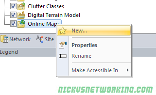
Starting a new Document
We’ll start by creating a new document:
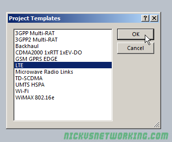
We’ll simulate an LTE network, so we’ll create it using the LTE project template.
Coordinate Reference
Before we can get to that we’re going to have to tell Atoll where we are and what datum we’re working in.
The data sets we’re working were provided by the Government, who use the Australian Geodetic Datum, and Christmas Island is in Zone 48.
We’ll select Document -> Properties
We’ll set the projection first.
Once that’s set we’ll set our display coordinates, this is what we’ll actually work in.
I’m using WGS 84 in the -xx.xxxxxx format, aka Lat & Long in decimal format.
Elevation
Elevation data is hugely important when network planning, your point-to-point links need LOS, and if your modeling / simulation doesn’t know there’s a hill or obstruction between the two sites, it’s not going to work.
There’s plenty of online sources for this data, some of which is paid, but others are provided free by Government agencies.
In this case the Digital Elevation Models for Christmas Island data can be downloaded from Geo-science Australia.
We’ll download the 5m DEM GDA94 UTM zone 48 Christmas Island.
The real reason I picked Christmas Island is that it’s DEM data is 16Mb instead of many Gigabytes and I didn’t want to wait for the download…
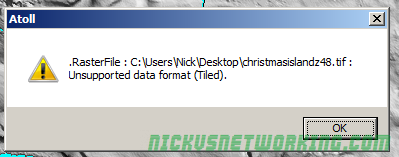
After a lot of messing around I found I couldn’t import the multi layered TIF provided by Geo Science Australia, Atoll gave me this error:
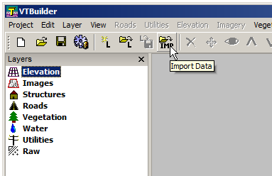
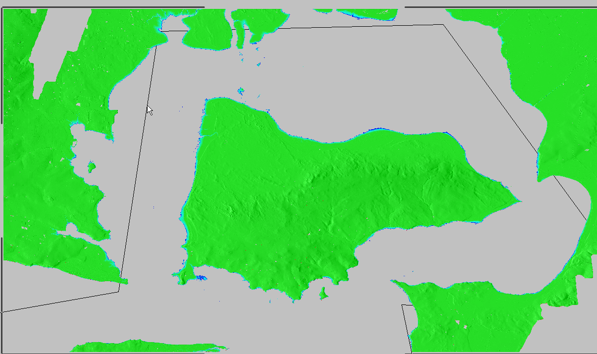
I found I could the TIFF formatted DEM files it in a package called VTBuilder, export it as a PNG and then import it into Atoll.
Using VTBuilder to convert DEMs in TIFF to PNG for importing into Atoll
To save some steps I’ve attached a copy of the converted file here.
You can then import the files straight into Atoll,
We’ll need to define what this dataset is, in our cases our Digital Elevation Models (aka Digital Terrain Models) contain Altitude information, so we’ll select Altitude (DTM)
We know from the metadata on the Geo Science Australia site we got the files from the resolution is 5m, so we’ll set pixel size to 5m (Each pixel represents 5 meters).
We’ll need a Geographic Coordinate, this is the Easting and Westing in relation to UTM Zone 48. The values are:
West
557999.9999999991
North
8849000
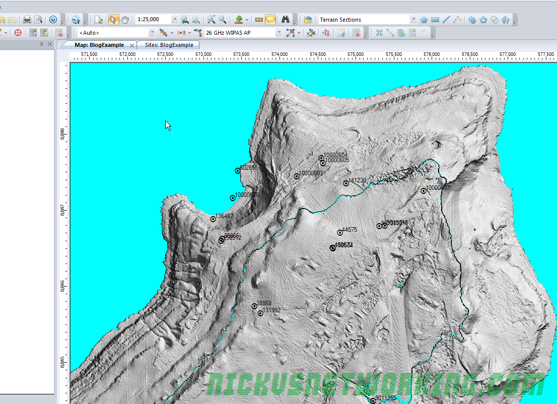
All going well you should see the imported topography showing up in Atoll.
I’ve noticed on the version I’m on I had some weirdness when zoomed out, if you try Zooming in to more than 1:10,000 you should see the terrain data. Not sure why this is but I’ve attached a copy of my Atoll config so far so you in case you get stuck with this.
We’ll download real world sites from the ACMA’s database,
I’ll use the cheat way by just looking it up on their map and exporting the data.
We’ll download the CSV file from the Map.
One thing we’ll need to change in the CSV is that when no Altitude is set for the site ACMA puts “undefined” which Atoll won’t be able to parse. So I’ve just opened it up in N++ and replaced undefined with 0.
I’ve attached a copy here for you to import / skip this step. Mastering messing with CSV is a super useful skill to have anyways, but that’s a topic for another day.
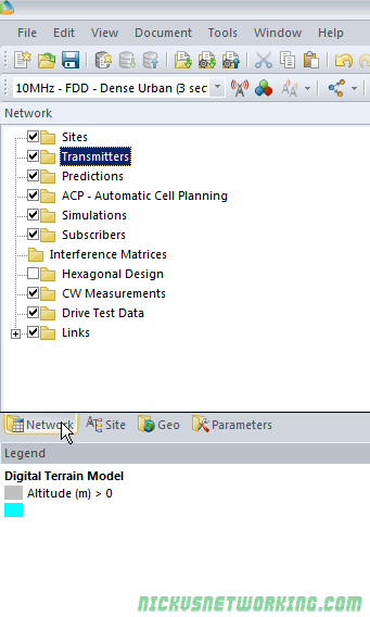
Next we’ll import the sites into Atoll, to define our sites, we’ll jump to the Network Tab and double click on Sites.
Now we’ll import our CSV file
Next we’ll need to define the fields for the import
All going well you’ll now have a populated site list.
Now if we go back to view we should see these points plotted.
Clutter
Forested areas, large bodies of water, urban sprawl, farmland, etc, all have different characteristics and will cause different interference patterns, refraction, shadow fading, etc.
Clutter Data is the classification of land use or land cover which impacts on RF propagation.
However this dataset doesn’t include Christmas Island. Really shot myself in the foot there, huh?
For examples’ sake we’ll import the terrain data again as clutter.
We’d normally define terrain classes, for example, this area is residential low rise etc, but as we don’t have areas set out we’ll skip that for now.
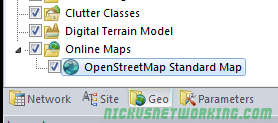
You can set different layer visibility by enabling and disabling layers in the Geo tab, in this case I’ve disabled my Digital Terrain Model layer and just left the Clutter Heights we just imported.
I got hit with the same Zoom bug here, not sure if it’s still loading in the background or something but the clutter data is only visible when zoomed to 1:10,000 or more, but after doing so you should see the clutter data:
So now we’ve got our environment stuff we can start to add some cell sites and model the propagation & expected signal levels throughout the island in the next post.
I recently began integrating IMS Authentication functions into PyHSS, and thought I’d share my notes / research into the authentication used by IMS networks & served by a IMS capable HSS.
There’s very little useful info online on AKAv1-MD5 algorithm, but it’s actually fairly simple to understand.
Authentication and Key Agreement (AKA) is a method for authentication and key distribution in a EUTRAN network. AKA is challenge-response based using symmetric cryptography. AKA runs on the ISIM function of a USIM card.
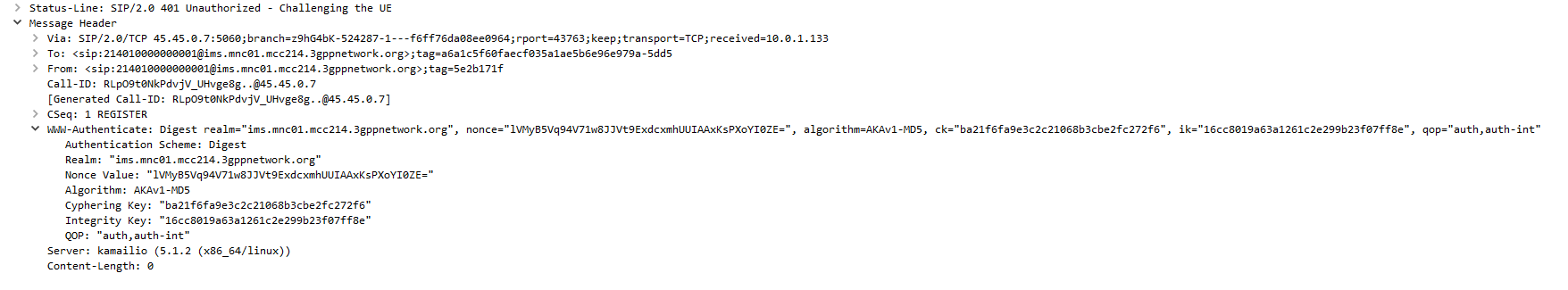
The Nonce field is the Base64 encoded version of the RAND value and concatenated with the AUTN token from our AKA response. (Often called the Authentication Vectors).
That’s it!
It’s put in the SIP 401 response by the S-CSCF and sent to the UE. (Note, the Cyperhing Key & Integrity Keys are removed by the P-CSCF and used for IPsec SA establishment.


