I do a lot of protocol testing, writing Diameter/PFCP/GTP-C etc, and spend a lot of time referencing the standards.
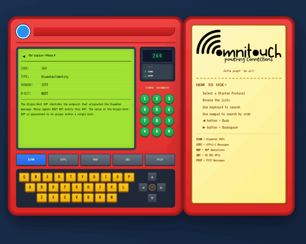
So I built this – Inspired by a 1990s video game / TV / Playing card franchise online reference tool, but rather than identifying pocket monsters, it’s identifying AVPs and stuff
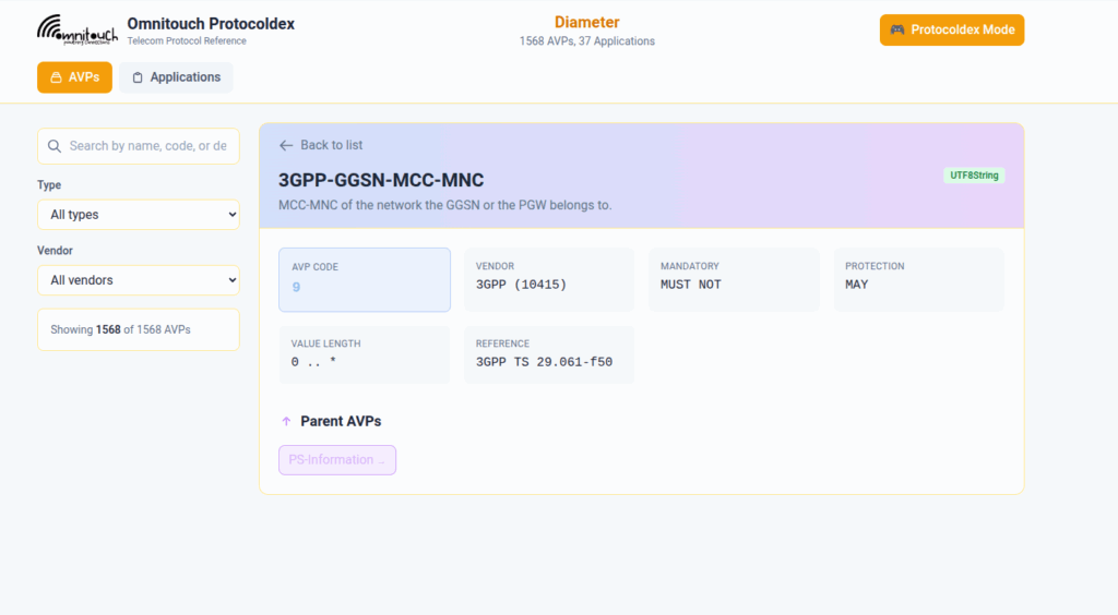
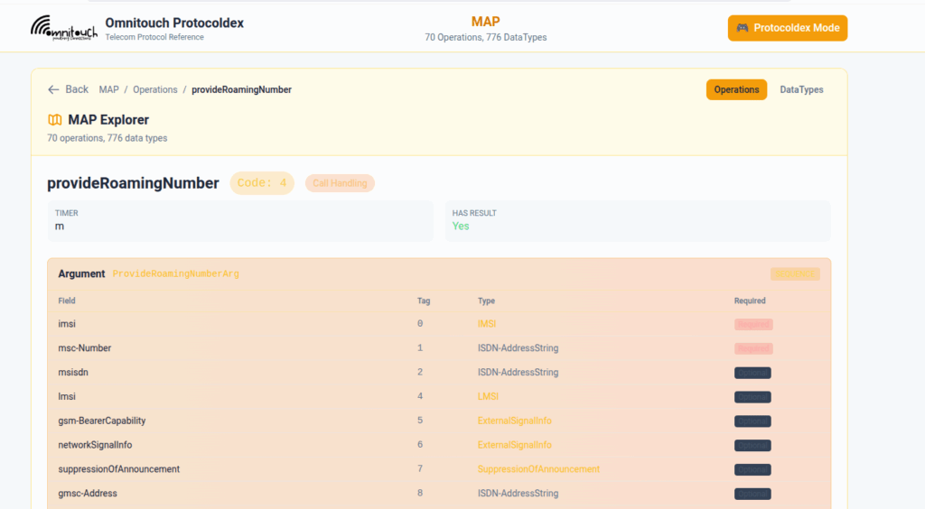
You can punch in the AVP code, AVP name, description, etc, for Diameter, PFCP, GTP-C, MAP or SBI and see all the details to go with it.
I’ve been using it a heap, hopefully some of you might find it useful:
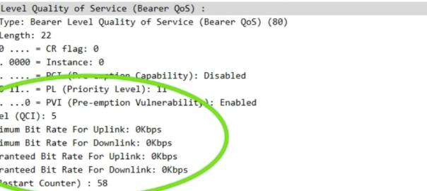
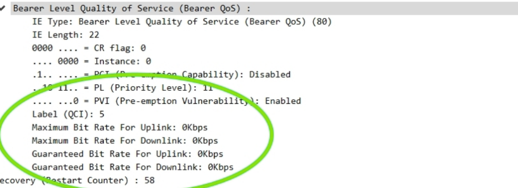
The other day I had a query about a roaming network that was sending Bearer Level QoS parameters in the Create Session Request to 0Kbps, up and down rather than populating the MBR values.
I knew for Guaranteed Bit Rate bearers that this was of course set, but for non GBR bearers (QCI 5 to 9) I figured this would be set the to MBR, but that’s not the case.
So what gives?
Well, according to TS 29.274:
For non-GBR bearers, both the UL/DL MBR and GBR should be set to zero.
So there you have it, if it’s not a QCI 1-4 bearer then these values are always 0.
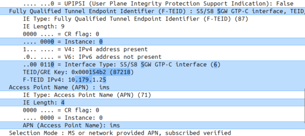
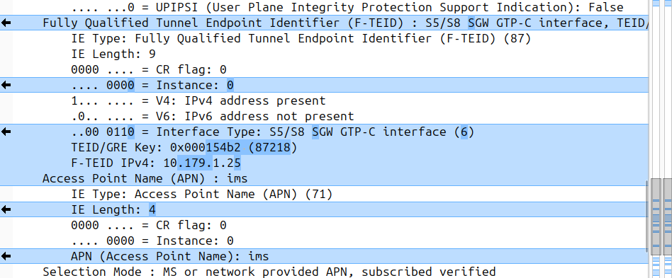
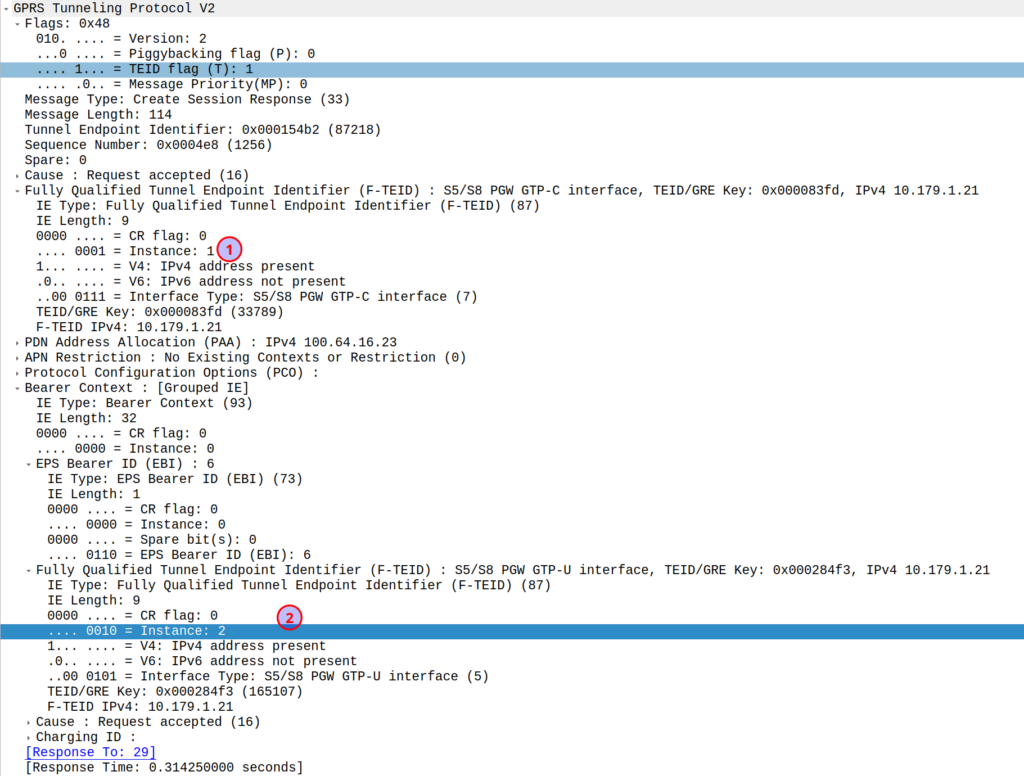
I was diffing two PCAPs the other day trying to work out what’s up, and noticed the Instance ID on a GTPv2 IE was different between the working and failing examples.
If more than one grouped information elements of the same type, but for a different purpose are sent with a message,
these IEs shall have different Instance values.
So if we’ve got two IEs of the same IE type (As we often do; F-TEIDs with IE Type 87 may have multiple instances in the same message each with different F-TEID interface types), then we differentiate between them by Instance ID.
The only exception to this rule is where we’ve got the same data, so if you’ve got one IE with the exact same values and purpose that exists twice inside the message.
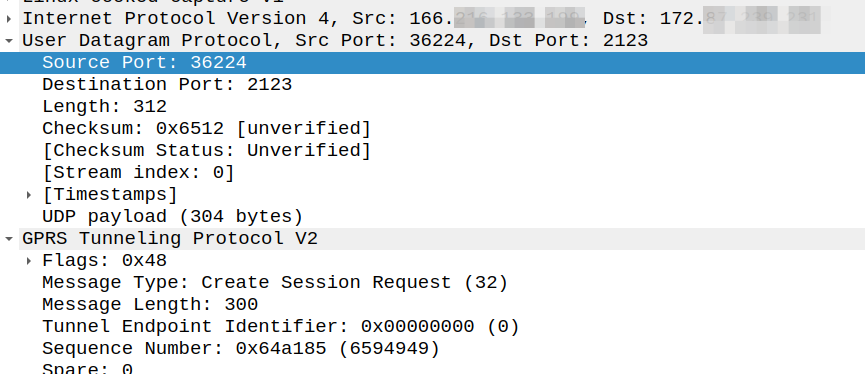
Ask anyone in the industry and they’ll tell you that GTPv2-C (aka GTP-C) uses port 2123, and they’re right, kinda.
Per TS 129.274 the Create Session Request should be sent to port 2123, but the source port can be any port:
The UDP Source Port for a GTPv2 Initial message is a locally allocated port number at the sending GTP entity.
So this means that while the Destination Port is 2123, the source port is not always 2123.
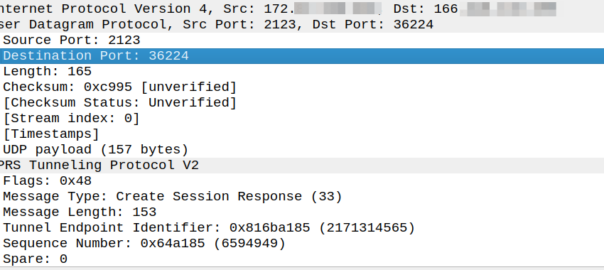
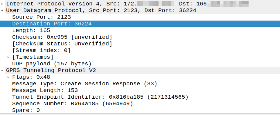
So what about a response to this? Our Create Session Response must go where?
Create Session request coming from 166.x.y.z from a random port 36225 Going to the PGW on 172.x.y.z port 2123
The response goes to the same port the request came on, so for the example above, as the source port was 36225, the Create Session Response must be sent to port 36225.
Because:
The UDP Destination Port value of a GTPv2 Triggered message and for a Triggered Reply message shall be the value of the UDP Source Port of the corresponding message to which this GTPv2 entity is replying, except in the case of the SGSN pool scenario.
But that’s where the association ends.
So if our PGW wants to send a Create Bearer Request to the SGW, that’s an initial message, so must go to port 2123, even if the Create Session Request came from a random different port.
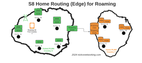
The S8 Home Routing approach for LTE Roaming works really well, as more and more operators are switching off their legacy circuit switched 2G/3G networks and shifting to LTE & VoLTE for roaming, we’re seeing more an more S8-HR deployments.
When LTE was being standardised in 2008, Local Breakout (LBO) and S8 Home Routing were both considered options for how roaming may look. Fast forward to today, and S8 Home routing is the only way roaming is done for modern deployments.
In light of this, there are some “best practices” in an “all S8 Home Routed” world, we’ve developed, that I thought I’d share.
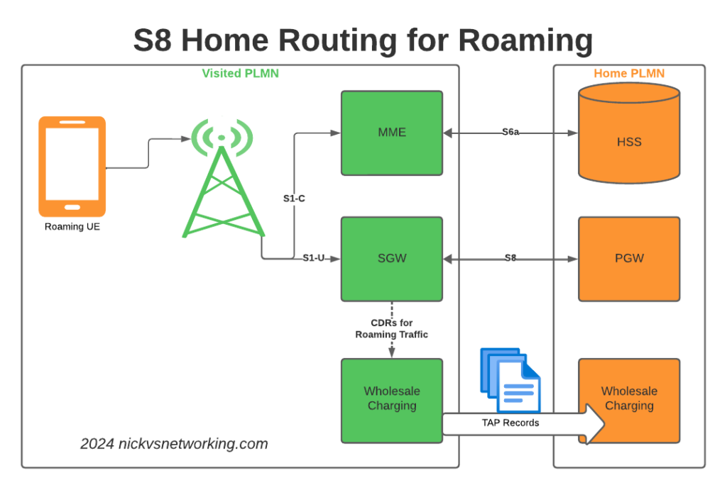
The Basics
When roaming, the SGW in the Visited Network, sends user traffic back to the PGW in the Home Network.
This means Online/Offline charging, IMS, PCRF, etc, is all done in the Home PLMN. As long as data packets can get from the SGW in the Visited PLMN to the PGW in the Home PLMN, and authentication flows from the Visited MME to the HSS in the Home PLMN, you’re golden.
The Constraints
Of course real networks don’t look as simple as this, in reality a roaming scenario for a visited network has a lot more nodes, which need to be
Building Distributed Packet Core & IMS
Virtualization (VNF / CNF) has led operators away from “big iron” hardware for Packet Core & IMS nodes, towards software based solutions, which in turn offer a lot more flexibility.
Best practice for design of User Plane is to keep the the latency down, by bringing the user plane closer to the user (the idea of “Edge” UPFs in 5GC is a great example of this), and the move away from “big iron” in central locations for SGW and PGW nodes has been the trend for the past decade.
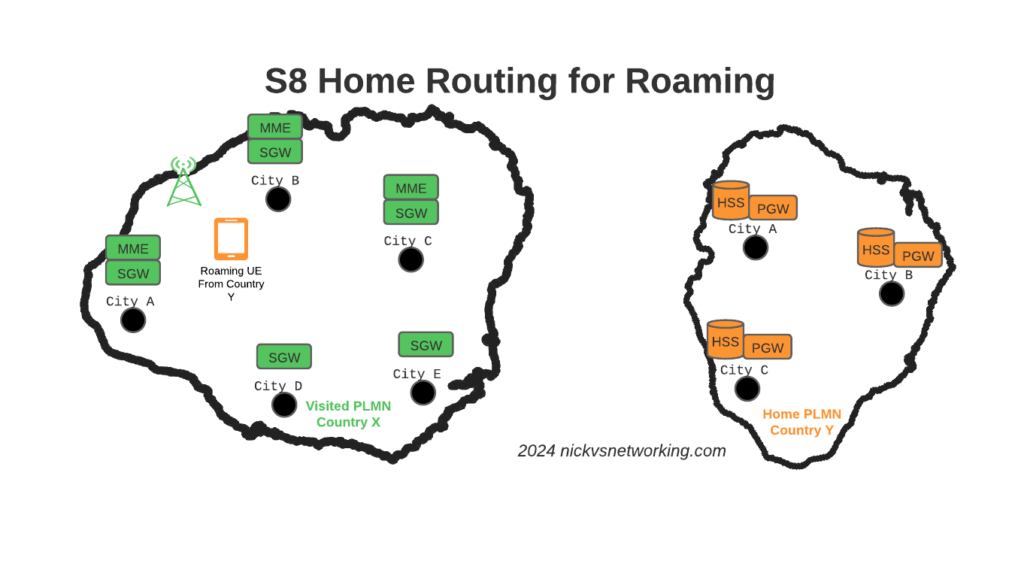
So to achieve these goals in the networks we build, we geographically distribute the core network.
This means we’ve got quite a few S-GW, P-GW, MME & HSS instances across the network. There’s some real advantages to this approach:
From a redundancy perspective this allows us to “spread the load” and build far more resilient networks. A network with 20 smaller HSS instances spread around the country, is far more resilient than 2 massive ones, regardless of how many power feeds or redundant disks it may have.
This allows us to be more resource efficient. MNOs have always provisioned excess capacity to cater for the loss of a node. If we have 2 MMEs serving a country, then each node has to have at least 50% capacity free, so if one MME were to fail, the other MME could handle the additional load it from it’s dead friend. This is costly for resources. Having 20 MMEs means each MME has to have 5% capacity free, to handle the loss of one MME in the pool.
It also forces our infrastructure teams to manage infrastructure “as cattle” rather than pets. These boxes don’t get names or lovingly crafted, they’re automatically spun up and destroyed without thinking about it.
For security, we only use internal IP addresses for the nodes in our packet core, this provides another layer of protection for the “crown jewels” of our network, so no one messing with BGP filtering can accidentally open the flood gates to our core, as one US operator learned leaving a GGSN open to the world leading to the private information for 100 million customers being leaked.
What this all adds to, is of course, the end user experience. For the end subscriber / customer, they get a better experience thanks to the reduced latency the connection provides, better uptime and faster call setup / SMS delivery, and less cost to deliver services.
I love this approach and could prothletise about it all day, but in a roaming context this presents some challenges.
The distributed networks we build are in a constant state of flux, new capacity is being provisioned in some areas, nodes things decommissioned in others, and our our core nodes are only reachable on internal IPs, so wouldn’t be reachable by roaming networks.
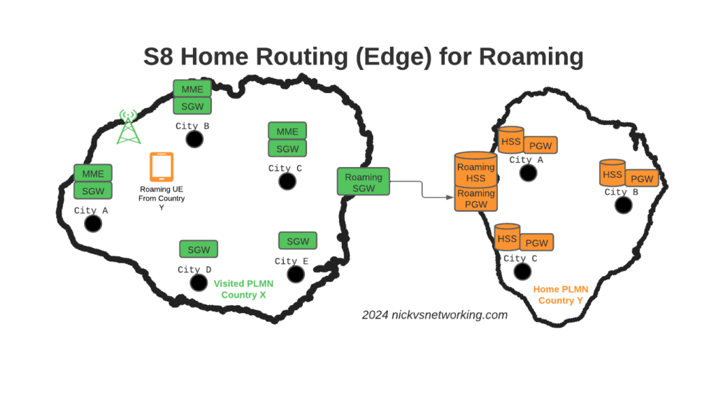
Our Distributed-Core Roaming Solution
To resolve this we’ve taken a novel approach, we’ve deployed a pair of S-GWs we call the “Roaming SGWs”, and a pair of P-GWs we call the “Roaming PGWs”, these do have public IPs, and are dedicated for use only by roaming traffic.
We really like this approach for a few reasons:
It allows us to be really flexible do what we want inside the network, without impacting roaming customers or operators who use our network for roaming. All the benefits I described from the distributed architectures can still be realised.
From a security standpoint, only these SGW/PGW pairs have public IPs, all the others are on internal IPs. This good for security – Our core network is the ‘crown jewels’ of the network and we only expose an edge to other providers. Even though IPX networks are supposed to be secure, one of the largest IPX providers had their systems breached for 5 years before it was detected, so being almost as distrustful of IPX traffic as Internet traffic is a good thing. This allows us to put these PGWs / SGWs at the “edge” of our network, and keep all our MMEs, as well as our on-net PGW and SGWs, on internal IPs, safe and secure inside our network.
For charging on the SGWs, we only need to worry about collecting CDRs from one set of SGWs (to go into the TAP files we use to bill the other operators), rather than running around hoovering up SGW CDRs from large numbers of Serving Gateways, which may get blown away and replaced without warning.
Of course, there is a latency angle to this, for international roaming, the traffic has to cross the sea / international borders to get to us. By putting it at the edge we’re seeing increased MOS on our calls, as the traffic is as close to the edge of the network as can be.
Caveat: Increased S11 Latency on Core Network sites over Satellite
This is probably not relevant to most operators, but some of our core network sites are fed only by satellite, and the move to this architecture shifted something: Rather than having latency on the S8 interface from the SGW to the PGW due to the satellite hop, we’ve got latency between the MME and the SGW due to the satellite hop.
It just shifts where in the chain the latency lies, but it did lead to us having to boost some timers in the MME and out of sequence deliver detection, on what had always been an internal interface previously.
Evolution to 5G Standalone Roaming
This approach aligns to the Home Routed options for 5G-SA roaming; UPF chaining means that the roaming traffic can still be routed, as seems to be the way the industry is going.
SA roaming is in its infancy, without widely deployed SA networks, we’re not going to see common roaming using SA for a good long while, but I’ll be curious to see if this approach becomes the de facto standard going forward.
Where to from here?
We’re pretty happy with this approach in the networks we’ve been building.
So far it’s made IREG testing easier as we’ve got two fixed points the IPX needs to hit (The DRAs and the SGWs) rather than a wide range of networks.
Operators with a vast number of APNs they need to drop into different VRFs may have to do some traffic engineering here – Our operations are generally pretty flat, but I can see where this may present some challenges for established operators shifting their traffic.
I’d be keen to hear if other operators are taking this approach and if they’ve run into any issues, or any issues others can see in this, feel free to drop a comment below.
As our subscribers are mobile, moving between base stations / cells, the destination of the incoming GTP-U packets needs to be updated every time the subscriber moves from one cell to another.
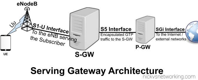
As we covered in the last post, the Packet Gateway (P-GW) handles decapsulating and encapsulating this traffic into GTP from external networks, and vise-versa. The Packet Gateway sends the traffic onto a Serving Gateway, that forwards the GTP-U traffic onto the eNodeB serving the user.
So why not just route the traffic from the Packet Gateway directly to the eNodeB?
As our users are inherently mobile, the signalling load to keep updating the destination of the incoming GTP-U traffic to the correct eNB, would put an immense load on the P-GW. So an intermediary gateway – the Serving Gateway (S-GW), is introduced.
The S-GW handles the mobility between cells, and takes the load of the P-GW. The P-GW just hands the traffic to a S-GW and let’s the S-GW handle the mobility.
It’s worth keeping in mind that most LTE connections are not “always on”. Subscribers (UEs) go into “Idle Mode”, in which the data connection and the radio connection is essentially paused, and able to be bought back at a moments notice (this allows us to get better battery life on the UE and better frequency utilisation).
When a user enters Idle Mode, an incoming packet needs to be buffered until the Subscriber/UE can get paged and come back online. Again this function is handled by the S-GW; buffering packets until the UE comes available then forwarding them on.
If you’re using an GSM / GPRS, UMTS, LTE or NR network, there’s a good chance all your data to and from the terminal is encapsulated in GTP.
GTP encapsulates user’s data into a GTP PDU / packet that can be redirected easily. This means as users of the network roam around from one part of the network to another, the destination IP of the GTP tunnel just needs to be updated, but the user’s IP address doesn’t change for the duration of their session as the user’s data is in the GTP payload.
One thing that’s a bit confusing is the TEID – Tunnel Endpoint Identifier.
Each tunnel has a sender TEID and transmitter TEID pair, as setup in the Create Session Request / Create Session Response, but in our GTP packet we only see one TEID.
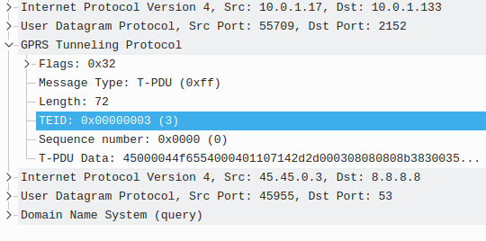
There’s not much to a GTP-U header; at 8 bytes in all it’s pretty lightweight. Flags, message type and length are all pretty self explanatory. There’s an optional sequence number, the TEID value and the payload itself.
So the TEID identifies the tunnel, but it’s worth keeping in mind that the TEID only identifies a data flow from one Network Element to another, for example eNB to S-GW would have one TEID, while S-GW to P-GW would have another TEID.
Each tunnel has two TEIDs, a sending TEID and a receiving TEID. For some reason (Minimize overhead on backhaul maybe?) only the sender TEID is included in the GTP header;
This means a packet that’s coming from a mobile / UE will have one TEID, while a packet that’s going to the same mobile / UE will have a different TEID.
Mapping out TIEDs is typically done by looking at the Create Session Request / Responses, the Create Session Request will have one TIED, while the Create Session Response will have a different TIED, thus giving you your TIED pair.
So far we’ve focused on building a plain “2G” (voice and SMS only) network, which was all consumers expected twenty years ago.
As the number of users accessing the internet through DSL, Dial Up & ISDN grew, the idea of getting this data “on the go” became more appealing. TCP/IP was becoming the dominant standard for networking, the first 802.11 WiFi spec had recently been published and demand for mobile data was growing.
There’s a catch however – TCP/IP was never designed to be mobile.
An IP address exists in a single location.
(Disclaimer: While you can “move” a subnet by advertising itself out in a different location via BGP peering relationships with other operators, it’s cumbersome, can only be done per /24 or larger, and most importantly it’s painfully slow. IPv6 has MIPv6 which attempts to fix some of these points, but that’s outside of this scope.)
GPRS addressed the mobility issue by having a single fixed point the IP Address is assigned to (the Gateway GPRS Support Node), which encapsulates IP traffic to/from a mobile user into GTP Packet (GPRS Tunnelling Protocol), like GRE or any of the other common routing encapsulation protocols, allowing the traffic to be rerouted to different destinations as the users move from being served by one BTS to another BTS.
So now we’ve got a method of encapsulating our data we’ve got to work out how to get that data out over the air.
BTS Time Slots
Way back when we were first setting up our BSC and adding our BTS(s) you will have configured timeslots for each BTS configured on your BSC.
Chances are if you’ve been following along with this tutorial, that you configured the first time slot (timeslot 0) as a CCCH+SDCCH4, meaning Common Control Channel and 4 standalone dedicated control channels, and all the subsequent timeslots (timeslot 1 – 7) as Traffic Channels (full rate) – TCH/F.
This works well if we’re only carrying voice, but to carry data we need timeslots to put the data traffic on.
For this we’ll re assign a timeslot we were using on our BSC as a voice traffic channel (TCH/F) as a PDCH – a Packet Data Channel.
This means that on the BSC your timeslot config will look something like this:
In the above example I’ve assigned two timeslots for Packet Data Channels,
The more timeslots you allocate for data, the more bandwidth available, but the fewer voice resources available.
(Most GSM networks today have few data timeslots as more recent RATs like 3G/4G are taking the data traffic, and GSM is used primarily for voice and low bandwidth M2M communications)
GPRS and EDGE
GPRS comes in two flavors, GPRS and EDGE.
GPRS (General Packet Radio Services) was the first of the two, standardised in R97, and allowed users to reach a downlink speeds of up to 171Kbps using GMSK on the air interface to encode the data.
Users quickly expected more speed, so EDGE (Enhanced Data rates for Global Evolution) was standardised, from a core perspective it was the same, but from a BTS / Air interface perspective it relied on 8PSK instead of GMSK allowed users to reach a blistering 384Kbps on the downlink.
These speeds are the theoretical maximums.
As the difference between GPRS and EDGE is encoding on the air interface, from a core perspective it’s treated the same way, however as our BTS gets all it’s brains from the BSC, we’ll need to specify if the BTS should use EDGE or GPRS it in the BSC’s BTS config.
BSC Config
On the BSC for each BTS we want to enable for packet data, we’ll need to define the parameters.
There’s two other values we’ll introduce when setting this up,
The first is NSEI – the Network Service Entity Identifier, which is the identifier of the BTS’s Packet Control Unit, like the cell identity.
The second value we’ll touch on is the BVCI – the BSSGP Virtual Connections Identifier, which is used for addressing between the BTS PCU and the SGSN.
I’ve been working on a ePDG for VoWiFi access to my IMS core.
This has led to a bit of a deep dive into GTP (easy enough) and GTPv2 (Bit harder).
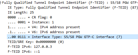
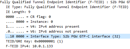
The Fully Qualified Tunnel Endpoint Identifier includes an information element for the Interface Type, identified by a two digit number.
Here we see S2b is 32
In the end I found the answer in 3GPP TS 29.274, but thought I’d share it here.
0
S1-U eNodeB GTP-U interface
1
S1-U SGW GTP-U interface
2
S12 RNC GTP-U interface
3
S12 SGW GTP-U interface
4
S5/S8 SGW GTP-U interface
5
S5/S8 PGW GTP-U interface
6
S5/S8 SGW GTP-C interface
7
S5/S8 PGW GTP-C interface
8
S5/S8 SGW PMIPv6 interface (the 32 bit GRE key is encoded in 32 bit TEID field and since alternate CoA is not used the control plane and user plane addresses are the same for PMIPv6)
9
S5/S8 PGW PMIPv6 interface (the 32 bit GRE key is encoded in 32 bit TEID field and the control plane and user plane addresses are the same for PMIPv6)
10
S11 MME GTP-C interface
11
S11/S4 SGW GTP-C interface
12
S10 MME GTP-C interface
13
S3 MME GTP-C interface
14
S3 SGSN GTP-C interface
15
S4 SGSN GTP-U interface
16
S4 SGW GTP-U interface
17
S4 SGSN GTP-C interface
18
S16 SGSN GTP-C interface
19
eNodeB GTP-U interface for DL data forwarding
20
eNodeB GTP-U interface for UL data forwarding
21
RNC GTP-U interface for data forwarding
22
SGSN GTP-U interface for data forwarding
23
SGW GTP-U interface for DL data forwarding
24
Sm MBMS GW GTP-C interface
25
Sn MBMS GW GTP-C interface
26
Sm MME GTP-C interface
27
Sn SGSN GTP-C interface
28
SGW GTP-U interface for UL data forwarding
29
Sn SGSN GTP-U interface
30
S2b ePDG GTP-C interface
31
S2b-U ePDG GTP-U interface
32
S2b PGW GTP-C interface
33
S2b-U PGW GTP-U interface
I also found how this data is encoded on the wire is a bit strange,
In the example above the Interface Type is 7,
This is encoded in binary which give us 111.
This is then padded to 6 bits to give us 000111.
This is prefixed by two additional bits the first denotes if IPv4 address is present, the second bit is for if IPv6 address is present.
Bit 1
Bit 2
Bit 3-6
IPv4 Address Present
IPv4 Address Present
Interface Type
1
1
000111
This is then encoded to hex to give us 87
Here’s my Python example;
interface_type = int(7)
interface_type = "{0:b}".format(interface_type).zfill(6)   #Produce binary bits
ipv4ipv6 = "10" #IPv4 only
interface_type = ipv4ipv6 + interface_type #concatenate the two
interface_type  = format(int(str(interface_type), 2),"x") #convert to hex
Let’s take a look at GTP, the workhorse of mobile user plane packet data.
This post covers all generations of mobile data (2.5 -> 5G), so I’m using generic terms.
GSM, UMTS, LTE & NR all have one protocol in common – GTP – The GPRS Tunneling Protocol.
So why do every generation of mobile data networks from GSM/GPRS in 2000, to 5G NR Standalone in 2020, rely on this one protocol for transporting user data?
So Why GTP?
GTP – the GPRS Tunnelling Protocol, is what encapsulates and tunnels IP packets from the internet / packet data network, to and from the User.
So why encapsulate the packets? What if the Base Station had access to the internet and routed the traffic to the users?
Let’s say we did that, we’d have to have large pools of IP addresses available at each Base Station and when a user connected they’d be assigned an IP Address and traffic for these users would be routed to the Base Station which would forward it onto the user.
This would work well until a user moves from one Base Station to another, when they’d have to get a new IP Address allocated.
TCP/IP was never designed to be mobile, an IP address only exists in a single location.
Breaking out traffic directly from a base station would have other issues, such as no easy way to enforce QoS or traffic policies, meter usage, etc.
How to fix IP’s lack of mobility? GTP.
GTP addressed the mobility issue by having a single fixed point the IP Address is assigned to (In GSM/GRPS/UMTS this is the Gateway GPRS Support Node, in LTE this is the P-GW and in 5G-SA this is the UPF), which encapsulates IP traffic to/from a mobile user into GTP Packet.
You can think of GTP like GRE or any of the other common encapsulation protocols, wrapping up the IP packets into a GTP packet which we can rerouted to different Base Stations as the users move from being served by one Base Station to another.
This easy redirecting / rerouting of user traffic is why GTP is used for NR (5G), LTE (4G), UMTS (3G) & GPRS (2.5G) architectures.
GTP Packets
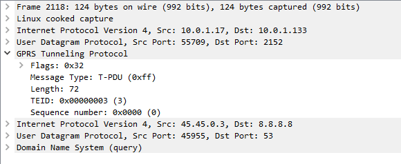
When looking at a GTP packet of user data you’d be forgiven for thinking nothing much goes on,
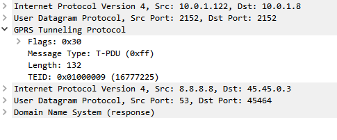
Example GTP packet containing a DNS query
Like in most tunneling / encapsulation protocols we’ve got the original network / protocol stack of IPv4 and UDP, and a payload of a GTP packet.
The packet itself is pretty bare bones, there’s flags, denoting a few basics like version number, the message type (T-PDU), the length of the GTP packet and it’s payload (used for delineating the end of the payload), a sequence number an a Tunnel Endpoint Identifier (TEID).
In the payload, we can see the network / protocol stack and application layer of the contents of the GTP packet.
From a mobility standpoint, the beauty of GTP is that it takes IP packets and puts them into a media stream of sorts, with out of band signalling, this means we can change the parameters of our GTP stream easily without touching the encapsulated IP Packet.
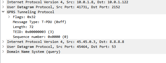
When a UE moves from one base station to another, all that has to happen is the destination the GTP packets are sent to is changed from the old base station to the new base station. This is signalled using GTP-C in GPRS/UMTS, GTPv2-C in LTE and HTTP in 5G-SA.
Traffic to and from the UE would look the same as the screenshot above, the only difference would be the first IPv4 address would be different, but the IPv4 address in the GTP tunnel would be the same.