Monthly Archives: September 2023

Australia’s East-West Microwave Link of the 1970s

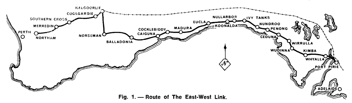
On July 9, 1970 a $10 million dollar program to link Australia from East to West via Microwave was officially opened.
Spanning over 2,400 kilometres, it connected Northam (to the east of Perth) to Port Pirie (north of Adelaide) and thus connected the automated telephone networks of Australia’s Eastern States and Western States together, to enable users to dial each other and share video live, across the country, for the first time.

In 1877, long before road and rail lines, the first telegraph line – a single iron wire, was spanned across the Nullabor to link Australia’s Eastern states with Western Australia.

By 1930 an open-wire voice link had been established between the two sides of the continent.
This was open-wire circuit was upgraded a rebuilt several times, to finally top out at 140 channels, but by the 1960s Australian Post Office (APO) engineers knew a higher bandwidth (broadband carrier) system was required if ever Standard Trunk Dialling (STD) was to be implemented so someone in Perth could dial someone in Sydney without going via an operator.

A few years earlier Melbourne and Sydney were linked via a 600 kilometre long coaxial cable route, so API engineers spent months in the Nullarbor desert surveying the soil conditions and came to the conclusion that a coaxial cable (like the recently opened Melbourne to Sydney Coaxial cable) was possible, but would be very difficult to achieve.

Instead, in 1966, Alan Hume, the Postmaster-General, announced that the decision had been made to construct a network of Microwave relay stations to span from South Australia to Western Australia.

In the 1930s microwave communications had spanned the English channel, by 1951 AT&T’s Long Lines microwave network had opened, spanning the continental United States. So by the 1960’s Microwave transmission networks were commonplace throughout Europe and the US and was thought to be fairly well understood.

But soon APO engineers soon realised that the unique terrain of the desert and the weather conditions of the Nullabor, had significant impacts on the transmission of Radio Waves. Again Research Labs staff went back to spend months in the desert measuring signal strength between test sites to better understand how the harsh desert environment would impact the transmission in order to overcome these impediments.

The length of the link was one of the longest ever attempted, longer than the distance from London to Moscow,

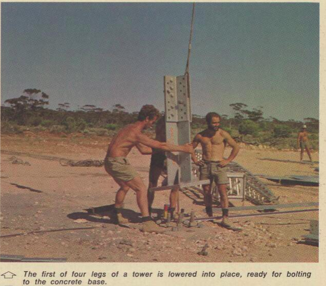
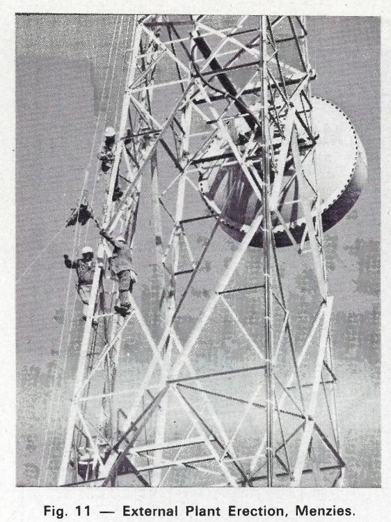
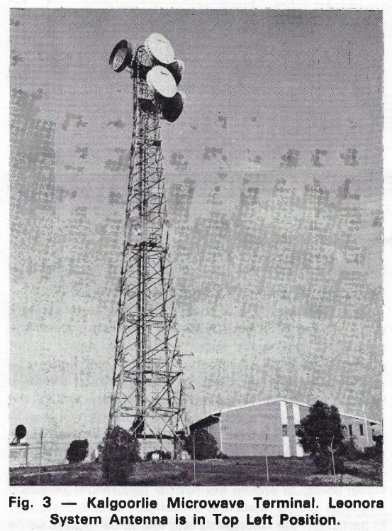
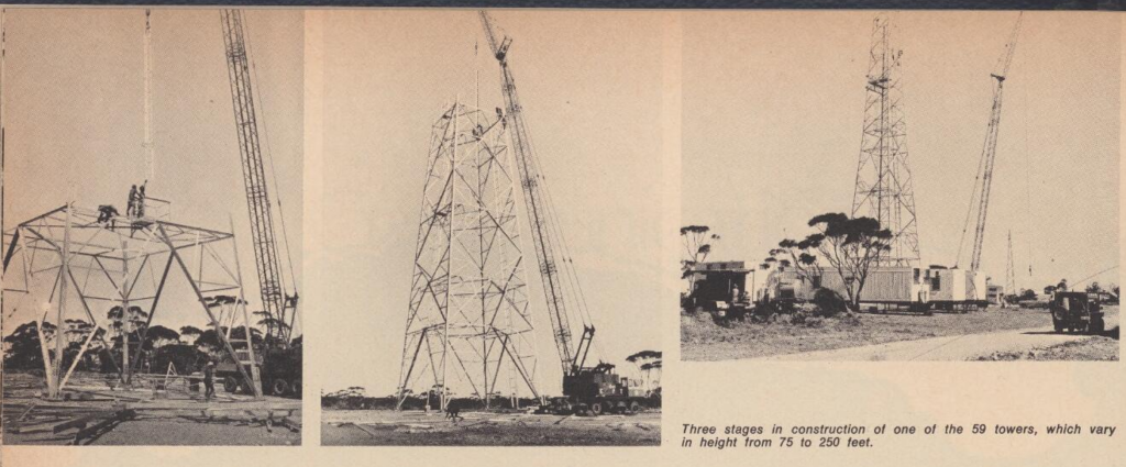
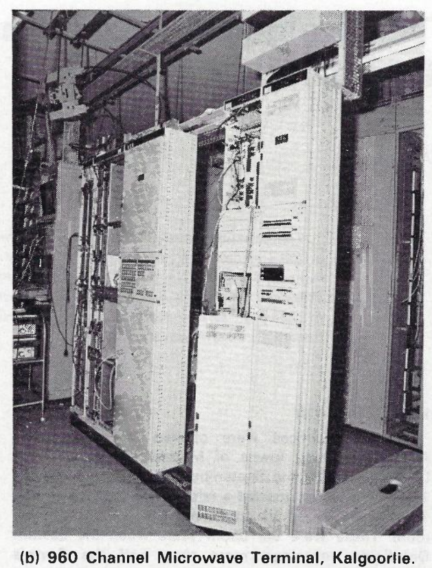
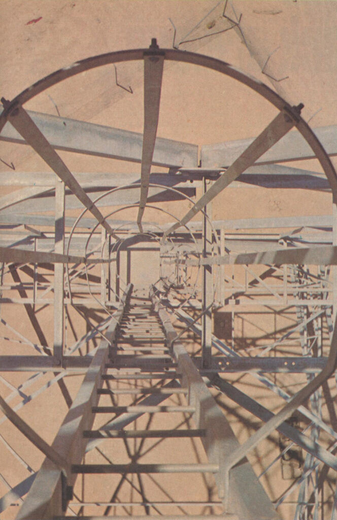
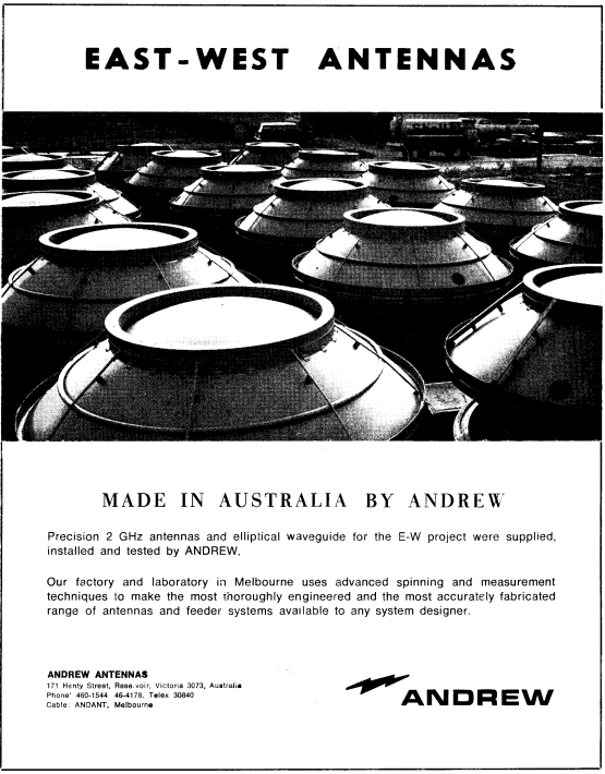
In the end it was decided that 59 towers with heights from 22 meters to 76 meters were to be built, topped off with 3.6m tall microwave dishes for relaying the messages between towers.

The towers themselves were to be built in a zig-zag pattern, to prevent overshooting microwave signals from interfering with signals for the next station in the chain.

Due to the remote nature of the repeater sites, for 43 of the 59 repeater sites had to be fully self sufficient in terms of power.

Initial planning saw the power requirements of the repeater sites to be limited to 500 watts, APO engineers looked at the available wind patterns and determined that combined with batteries, wind generators could keep these sites online year round, without the need for additional power sources. Unfortunately this 500 watt power consumption target quickly tripled, and diesel generators were added to make up any shortfall on calm days.

The addition of the Diesel gensets did not in any way reduce the need to conserve power – the more Diesel consumed, the more trips across the desert to refuel the diesel generators would be required, so the constant need to keep power to a minimum was one of the key restraints in the project.

The designs of these huts were reused after the project for extreme temperature equipment housings, including one reused by Broadcast Australia seen in Marble Barr – The hottest town in Australia.

Active cooling systems (Like Air Conditioning) were out of the question due to being too power hungry. APO engineers knew that the more efficient equipment they could use, the less heat they would produce, and the more efficient the system would be, so solid state (transistorised devices) were selected for the 2Ghz transmission equipment, instead of valves which would have been more power-hungry and produced more heat.

The reduced power requirement of the fully transistorized radio equipment meant that wind-supplied driven generators could provide satisfactory amounts of power provided that the wind characteristics of the site were suitable.

THE TELECOMMUNICATION JOURNAL OF AUSTRALIA / Volume 21 / Issue 21 / February 1971

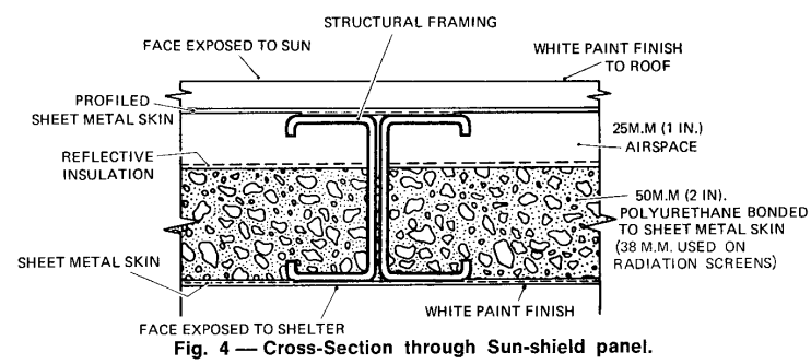
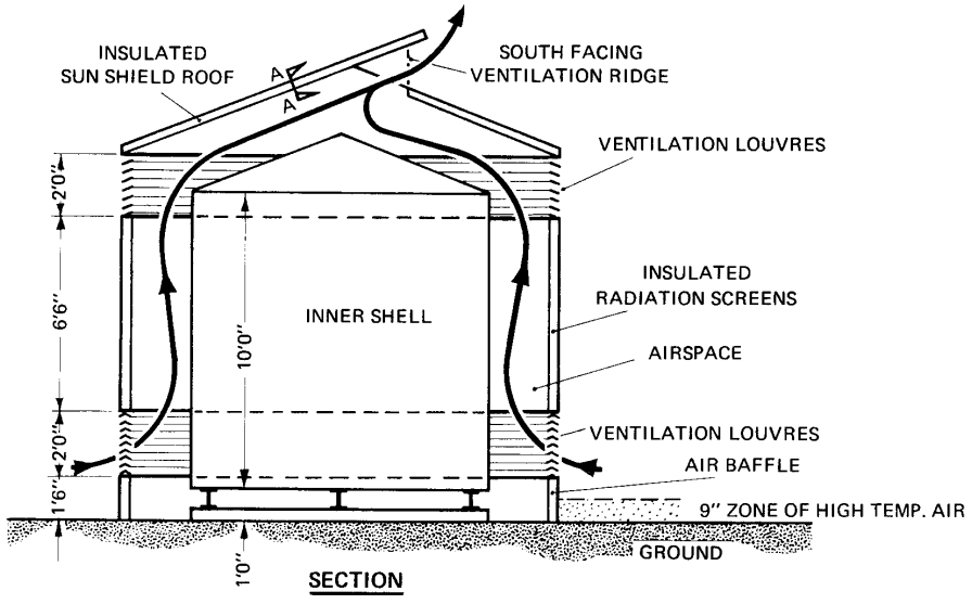
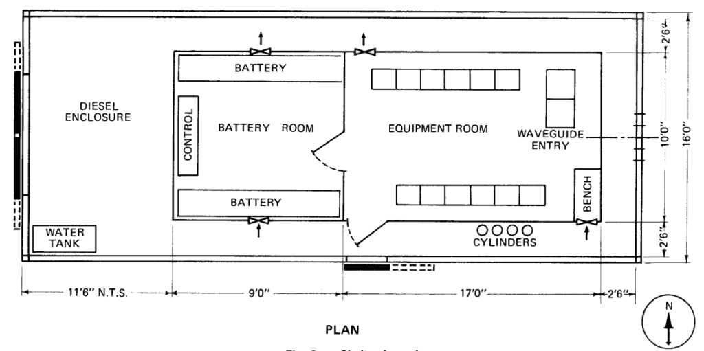
So forced to use passive cooling methods, the engineers on the project designed the repeater huts to cleverly utilize ventilation and the orientation of the huts to keep them as cool as possible.

Construction was rough, but in just under 2 years the teams had constructed all 59 towers and the associated equipment huts to span the desert.

When the system first opened for service in July 1970, live TV programs could be simulcast on both sides of the country, for the first time, and someone in Perth could pick up the phone and call someone in Melbourne directly (previously this would have gone through an operator).

PMG Engineers designed a case to transport the fragile equipment spares – That resided in the back of a Falcon XR Station Wagon

The system offered 1+1 redundancy, and capacity for 600 circuits, split across up to 6 radio bearers, and a bearer could be dedicated at times to support TV transmissions, carried on 5 watt (2 watt when modulated) carriers, operating at 1.9 to 2.3Ghz.

By linking the two sides of Australia, Telecom opened up the ability to have a single time source distributed across the country, the station in Lyndhurst in Victoria, created the 100 “microseconds” signal generated by a VNG, that was carrier across the link.

Looking down one of the towers

Unlike AT&T’s Long Lines network, which lasted until after MCI, deregulation and the breakup off the Bell System, the East-West link didn’t last all that long.

By 1981, Telecom Australia (No longer APO) had installed their first experimental optic fibre cable between Clayton and Springvale, and fibre quickly became the preferred method for broadband carrier circuits between exchanges.

By 1987, Melbourne and Sydney were linked by fibre, and the benefits of fibre were starting to be seen more broadly, and by 1989, just under 20 years since the original East-West Microwave system opened, Telecom Australia completed a 2373 kilometre long / 14 fibre cable from Perth to Adelaide, and Optus followed in 1993.

This effectively made the microwave system redundant. Fibre provided a higher bandwidth, more reliable service, that was far cheaper to operate due to decreased power requirements. And so piece by piece microwave hops were replaced with fibre optic cables.

I’m not clear on which was the last link to be switched off (If you do know please leave a comment or drop me a message), but eventually at some point in the late 1980s or early 1990s, the system was decommissioned.

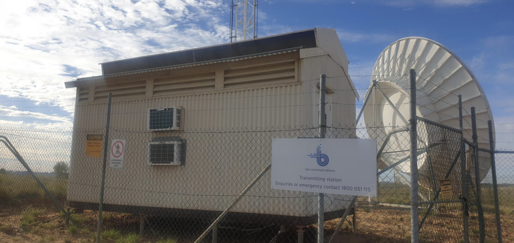
Many of the towers still stand today and carry microwave equipment on them, but it is a far cry from what was installed in the late 1960s.

Advertisement from Andrew Antennas

References

East-west microwave link opening (Press Release)

Walkabout.Vol. 35 No. 6 (1 June 1969) – Communications Across the Nullabor

$8 Million Trans-continental link

ABC Goldfields-Esperance – Australia’s first live national television broadcast

APO – Newsletter ‘New East-West Trunks System’

TelevisionAU.com 50 years since Project Australia

Whirlpool Post

TJA Article on spur to Lenora

VoLTE / IMS – Analysis Challenge

It’s challenge time, this time we’re going to be looking at an IMS PCAP, and answering some questions to test your IMS analysis chops!

Here’s the packet capture:

Easy Questions

  • What QCI value is used for the IMS bearer?
  • What is the registration expiry?
  • What is the E-UTRAN Cell ID the Subscriber is served by?
  • What is the AMBR of the IMS APN?

Intermediate Questions

  • Is this the first or subsequent registration?
  • What is the Integrity-Key for the registration?
  • What is the FQDN of the S-CSCF?
  • What Nonce value is used and what does it do?
  • What P-CSCF Addresses are returned?
  • What time would the UE need to re-register by in order to stay active?
  • What is the AA-Request in #476 doing?
  • Who is the(opens in a new tab)(opens in a new tab)(opens in a new tab) OEM of the handset?
  • What is the MSISDN associated with this user?

Hard Questions

  • What port is used for the ESP data?
  • Which encryption algorithm and algorithm is used?
  • How many packets are sent over the ESP tunnel to the UE?
  • Where should SIP SUBSCRIBE requests get routed?
  • What’s the model of phone?

The answers for each question are on the next page, let me know in the comments how you went, and if there’s any tricky ones!

Mobile IPv6 Tax?

Recently a Tweet from Dean Bubly got me thinking about how data is charged in cellular:

In the cellular world, subscribers are charged for data from the IP, transport and applications layers; this means you pay for the IP header, you pay for the TCP/UDP header, and you pay for the contents (the cat videos it contains).

This also means if an operator moves mobile subscribers from IPv4 to IPv6, there’s an extra 20 bytes the customer is charged for for every packet sent / received, which the customer is charged for – This is because the IPv6 header is longer than the IPv4 header.

Source: ServerFault - https://serverfault.com/questions/547768/ipv4-header-vs-ipv6-header-size

In most cases, mobile subs don’t get a choice as to if their connection is IPv4 or IPv6, but on a like for like basis, we can say that if a customer moves is on IPv6 every packet sent/received will have an extra 20 bytes of data consumed compared to IPv4.

This means subscribers use more data on IPv6, and this means they get charged for more data on IPv6.

For IoT applications, light users and PAYG users, this extra 20 bytes per packet could add up to something significant – But how much?

We can quantify this, but we’d need to know the number of packets sent on average, and the quantity of the data transferred, because the number of packets is the multiplier here.

So for starters I’ve left a phone on the desk, it’s registered to the network but just sitting in Idle mode – This is an engineering phone from an OEM, it’s just used for testing so doesn’t have anything loaded onto it in terms of apps, it’s not signed into any applications, or checking in the background, so I thought I’d try something more realistic.

So to get a clearer picture, I chucked a SIM in my regular everyday phone I use personally, registered it to the cellular lab I have here. For the next hour I sniffed the GTP traffic for the phone while it was sitting on my desk, not touching the phone, and here’s what I’ve got:

Overall the PCAP includes 6,417,732 bytes of data, but this includes the transport and GTP headers, meaning we can drop everything above it in our traffic calculations.

Everything except the data encapsulated in GTP can be dropped

For this I’ve got 14 bytes of ethernet, 20 bytes IP, 8 bytes UDP and 5 bytes for TZSP (this is to copy the traffic from the eNB to my local machine), then we’ve got the transport from the eNB to the SGW, 14 bytes of ethernet again, 20 bytes of IP , 8 bytes of UDP and 8 bytes of GTP then the payload itself. Phew.
All this means we can drop 97 bytes off every packet.

We have 16,889 packets, 6,417,732 bytes in total, minus 97 bytes from each gives us 1,638,233 of headers to drop (~1.6MB) giving us a total of 4.556 MB traffic to/from the phone itself.

This means my Android phone consumes 4.5 MB of cellular data in an hour while sitting on the desk, with 16,889 packets in/out.

Okay, now we’re getting somewhere!

So now we can answer the question, if each of these 16k packets was IPv6, rather than IPv4, we’d be adding another 20 bytes to each of them, 20 bytes x 16,889 packets gives 337,780 bytes (~0.3MB) to add to the total.

If this traffic was transferred via IPv6, rather than IPv4, we’d be looking at adding 20 bytes to each of the 16,889 packets, which would equate to 0.3MB extra, or about 7% overhead compared to IPv4.

But before you go on about what an outrage this IPv6 transport is, being charged for those extra bytes, that’s only one part of the picture.

There’s a reason operators are finally embracing IPv6, and it’s not to put an extra 7% of traffic on the network (I think if you asked most capacity planners, they’d say they want data savings, not growth).

IPv6 is, for lack of a better term, less rubbish than IPv4.

There’s a lot of drivers for IPv6, and some of these will reduce data consumption.
IPv6 is actually your stuff talking directly to the remote stuff, this means that we don’t need to rely on NAT, so no need to do NAT keepalives, and opening new sessions, which is going to save you data. If you’re running apps that need to keep a connection to somewhere alive, these data savings could negate your IPv6 overhead costs.

Will these potential data savings when using IPv6 outweigh the costs?

That’s going to depend on your use case.

If you’ve extremely bandwidth / data constrained, for example, you have an IoT device on an NTN / satellite connection, that was having to Push data every X hours via IPv4 because you couldn’t pull data from it as it had no public IP, then moving it to IPv6 so you can pull the data on the public IP, on demand, will save you data. That’s a win with IPv6.

If you’re a mobile user, watching YouTube, getting push notifications and using your phone like a normal human, probably not, but if you’re using data like a normal user, you’ve probably got a sizable data allowance that you don’t end up fully consuming, and the extra 20 bytes per packet will be nothing in comparison to the data used to watch a 2k video on your small phone screen.

DNS – TCP or UDP?

Ask someone with headphones and a lanyard in the halls of a datacenter what transport does DNS use, there’s a good chance the answer you’d get back is UDP Port 53.

But not always!

In scenarios where the DNS response is large (beyond 512 bytes) a DNS query will shift over to TCP for delivery.

How does the client know when to shift the request to TCP – After all, the DNS server knows how big the response is, but the client doesn’t.

The answer is the Truncated flag, in the response.

The DNS server sends back a response, but with the Truncated bit set, as per RFC 1035:

TC TrunCation – specifies that this message was truncated due to length greater than that permitted on the transmission channel.

RFC 1035

Here’s an example of the truncated bit being set in the DNS response.

The DNS client, upon receiving a response with the truncated bit set, should run the query again, this time using TCP for the transport.

One prime example of this is DNS NAPTR records used for DNS in roaming scenarios, where the response can quite often be quite large.

If it didn’t move these responses to TCP, you’d run the risk of MTU mismatches dropping DNS. In that half of my life has been spent debugging DNS issues, and the other half of my life debugging MTU issues, if I had MTU and DNS issues together, I’d be looking for a career change…