Recently I’ve been doing some work with FreeSWITCH as an IMS Conference Factory, I’ve written a bit about it before in this post on using FreeSWITCH with the AMR codec.
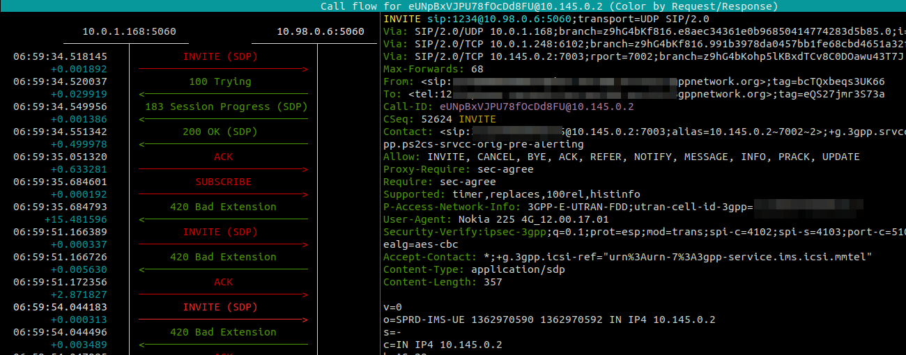
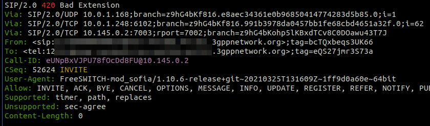
Pretty early on in my testing I faced a problem with subsequent in-dialog responses, like re-INVITEs used for holding the calls.
Every subsequent message, was getting a “420 Bad Extension” response from FreeSWITCH.
The ReINVITEThe 420 Bad Extension Response
So what didn’t it like and why was FreeSWITCH generating 420 Bad Extension Responses to these subsequent messages?
Well, the “Extensions” FreeSWITCH is referring to are not extensions in the Telephony sense – as in related to the Dialplan, like an Extension Number to identify a user, but rather the Extensions (as in expansions) to the SIP Protocol introduced for IMS.
The re-INVITE contains a Require header with sec-agree which is a SIP Extension introduced for IMS, which FreeSWITCH does not have support for, and the re-INVITE says is required to support the call (Not true in this case).
Using a Kamailio based S-CSCF means it is easy to strip these Headers before forwarding the requests onto the Application Server, which is what I’ve done, and bingo, no more errors!
So you have a VoIP service and you want to rate the calls to charge your customers?
You’re running a mobile network and you need to meter data used by subscribers?
Need to do least-cost routing?
You want to offer prepaid mobile services?
Want to integrate with Asterisk, Kamailio, FreeSWITCH, Radius, Diameter, Packet Core, IMS, you name it!
Well friends, step right up, because today, we’re talking CGrates!
So before we get started, this isn’t going to be a 5 minute tutorial, I’ve a feeling this may end up a big multipart series like some of the others I’ve done. There is a learning curve here, and we’ll climb it together – but it is a climb.
Installation
Let’s start with a Debian based OS, installation is a doddle:
We’re going to use Redis for the DataDB and MariaDB as the StorDB (More on these concepts later), you should know that other backend options are available, but for keeping things simple we’ll just use these two.
Next we’ll get the database and config setup,
cd /usr/share/cgrates/storage/mysql/
./setup_cgr_db.sh root CGRateS.org localhost
cgr-migrator -exec=*set_versions -stordb_passwd=CGRateS.org
Lastly we’ll clone the config files from the GitHub repo:
In its simplest form, rating is taking a service being provided and calculating the cost for it.
The start of this series will focus on voice calls (With SMS, MMS, Data to come), where the callingparty (The person making the call) pays, so let’s imagine calling a Mobile number (Starting with 614) costs $0.22 per minute.
To perform rating we need to determine the Destination, the Rate to be applied, and the time to charge for.
For our example earlier, a call to a mobile (Any number starting with 614) should be charged at $0.22 per minute. So a 1 minute call will cost $0.22 and a 2 minute long call will cost $0.44, and so on.
We’ll also charge calls to fixed numbers (Prefix 612, 613, 617 and 617) at a flat $0.20 regardless of how long the call goes for.
So let’s start putting this whole thing together.
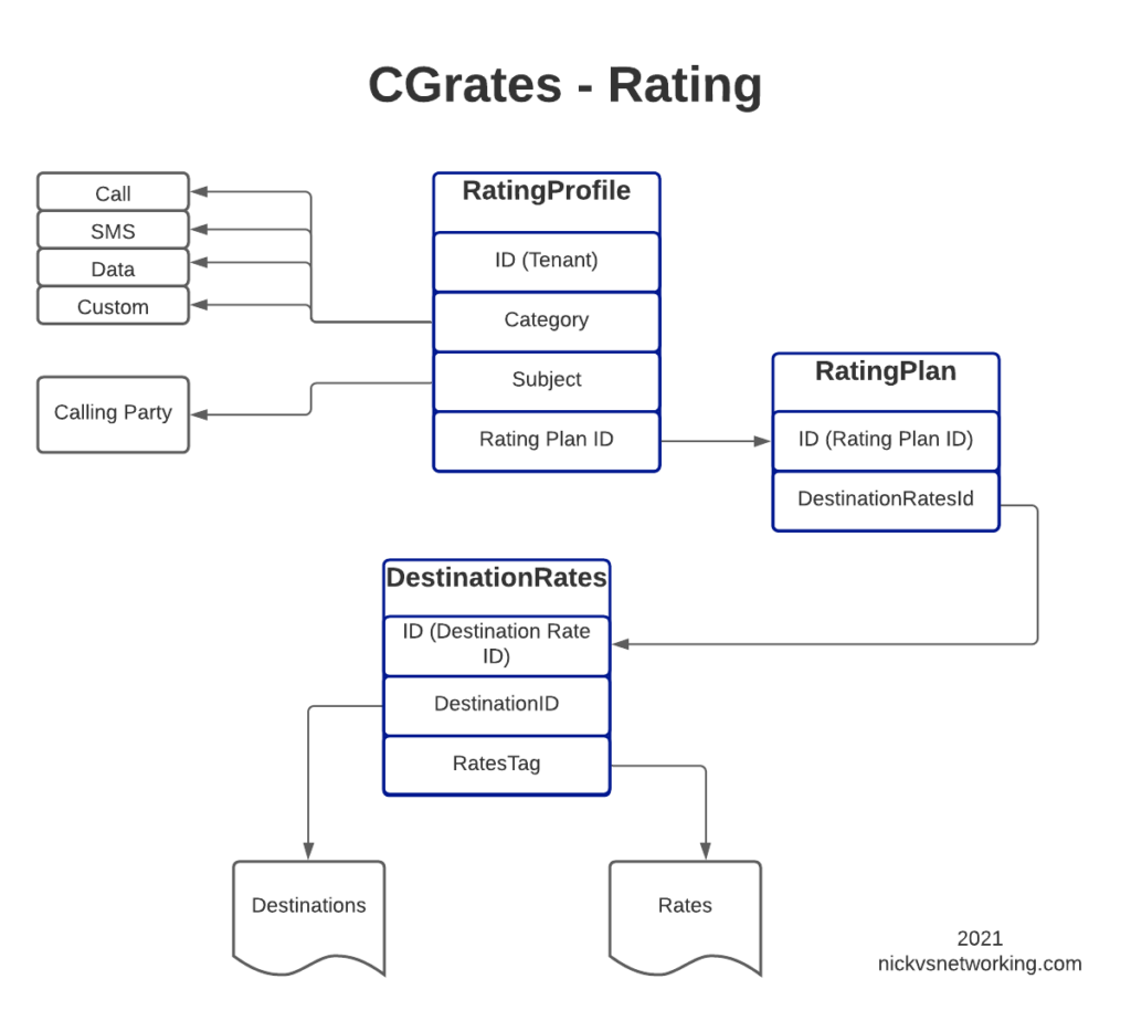
Introduction to RALs
RALs is the component in CGrates that takes care of Rating and Accounting Logic, and in this post, we’ll be looking at Rating.
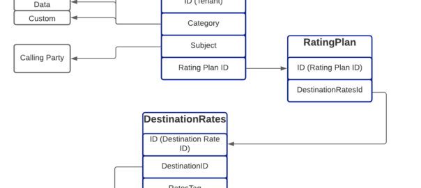
The rates have hierarchical structure, which we’ll go into throughout this post. I took my notepad doodle of how everything fits together and digitized it below:
Destinations
Destinations are fairly simple, we’ll set them up in our Destinations.csv file, and it will look something like this:
Each entry has an ID (referred to higher up as the Destination ID), and a prefix.
Also notice that some Prefixes share an ID, for example 612, 613, 617 & 618 are under the Destination ID named “DST_AUS_Fixed”, so a call to any of those prefixes would match DST_AUS_Fixed.
Rates
Rates define the price we charge for a service and are defined by our Rates.csv file.
This is nice and clean, a 1 second call costs $0.25, a 60 second call costs $0.25, and a 61 second call costs $0.50, and so on.
This is the standard billing mechanism for residential services, but it does not pro-rata the call – For example a 1 second call is the same cost as a 59 second call ($0.25), and only if you tick over to 61 seconds does it get charged again (Total of $0.50).
Per Second Billing
If you’re doing a high volume of calls, paying for a 3 second long call where someone’s voicemail answers the call and was hung up, may seem a bit steep to pay the same for that as you would pay for 59 seconds of talk time.
Instead Per Second Billing is more common for high volume customers or carrier-interconnects.
This means the rate still be set at $0.25 per minute, but calculated per second.
So the cost of 60 seconds of call is $0.25, but the cost of 30 second call (half a minute) should cost half of that, so a 30 second call would cost $0.125.
How often we asses the charging is defined by the RateIncrement parameter in the Rate Table.
We could achieve the same outcome another way, by setting the RateIncriment to 1 second, and the dividing the rate per minute by 60, we would get the same outcome, but would be more messy and harder to maintain, but you could think of this as $0.25 per minute, or $0.004166667 per second ($0.25/60 seconds).
Flat Rate Billing
Another option that’s commonly used is to charge a flat rate for the call, so when the call is answered, you’re charged that rate, regardless of the length of the call.
Regardless if the call is for 1 second or 10 hours, the charge is the same.
DestinationID – Refers to the DestinationID defined in the Destinations.csv file
RatesTag – Referes to the Rate ID we defined in Rates.csv
RoundingMethod – Defines if we round up or down
RoundingDecimals – Defines how many decimal places to consider before rounding
MaxCost – The maximum cost this can go up to
MaxCostStrategy – What to do if the Maximum Cost is reached – Either make the rest of the call Free or Disconnect the call
So for each entry we’ll define an ID, reference the Destination and the Rate to be applied, the other parts we’ll leave as boilerplate for now, and presto. We have linked our Destinations to Rates.
Rating Plans
We may want to offer different plans for different customers, with different rates.
DestinationRatesId (As defined in DestinationRates.csv)
TimingTag – References a time profile if used
Weight – Used to determine what precedence to use if multiple matches
So as you may imagine we need to link the DestinationRateIDs we just defined together into a Rating Plan, so that’s what I’ve done in the example above.
Rating Profiles
The last step in our chain is to link Customers / Subscribers to the profiles we’ve just defined.
How you allocate a customer to a particular Rating Plan is up to you, there’s numerous ways to approach it, but for this example we’re going to use one Rating Profile for all callers coming from the “cgrates.org” tenant:
Category is used to define the type of service we’re charging for, in this case it’s a call, but could also be an SMS, Data usage, or a custom definition.
Subject is typically the calling party, we could set this to be the Caller ID, but in this case I’ve used a wildcard “*any”
ActivationTime allows us to define a start time for the Rating Profile, for example if all our rates go up on the 1st of each month, we can update the Plans and add a new entry in the Rating Profile with the new Plans with the start time set
RatingPlanID sets the Rating Plan that is used as we defined in RatingPlans.csv
Loading the Rates into CGrates
At the start we’ll be dealing with CGrates through CSV files we import, this is just one way to interface with CGrates, there’s others we’ll cover in due time.
CGRates has a clever realtime architecture that we won’t go into in any great depth, but in order to load data in from a CSV file there’s a simple handy tool to run the process,
Obviously you’ll need to replace with the folder you cloned from GitHub.
Trying it Out
In order for CGrates to work with Kamailio, FreeSWITCH, Asterisk, Diameter, Radius, and a stack of custom options, for rating calls, it has to have common mechanisms for retrieving this data.
CGrates provides an API for rating calls, that’s used by these platforms, and there’s a tool we can use to emulate the signaling for call being charged, without needing to pickup the phone or integrate a platform into it.
The tenant will need to match those defined in the RatingProfiles.csv, the Subject is the Calling Party identity, in our case we’re using a wildcard match so it doesn’t matter really what it’s set to, the Destination is the destination of the call, AnswerTime is time of the call being answered (pretty self explanatory) and the usage defines how many seconds the call has progressed for.
The output is a JSON string, containing a stack of useful information for us, including the Cost of the call, but also the rates that go into the decision making process so we can see the logic that went into the price.
So have a play with setting up more Destinations, Rates, DestinationRates and RatingPlans, in these CSV files, and in our next post we’ll dig a little deeper… And throw away the CSVs all together!
This is part of a series of posts looking into SS7 and Sigtran networks. We cover some basic theory and then get into the weeds with GNS3 based labs where we will build real SS7/Sigtran based networks and use them to carry traffic.
So, all going well at this point in the tutorial you’ve got your lab setup with SS7 links between our simulated countries, but we haven’t dug too deep into what’s going on.
Most of the juicy stuff happens in the higher layers, but in this post we’ll look at the Data-Link layer for SS7.
In TDM based SS7 networks, Data Link layer is handled by a layer called “MTP2” – Message Transfer Part 2, which is responsible for flow control and ensuring guaranteed delivery between two points on the network.
MTP2 provides the services you’d typically expect at the Data Link Layer; link alignment, CRC generation/verification, end to end transmission between two points, flow control and sequence verification, etc.
MTP2 is responsible for making the connection between two points capable of carrying those far more interesting upper layers, but it’s really important, particularly when we talk about SIGTRAN/SS7 over IP, to understand how this can be done, so you can understand how the networks fit together.
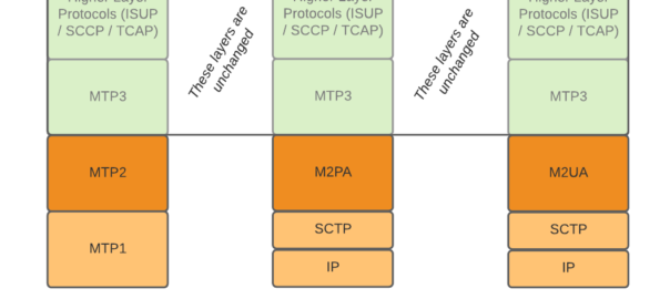
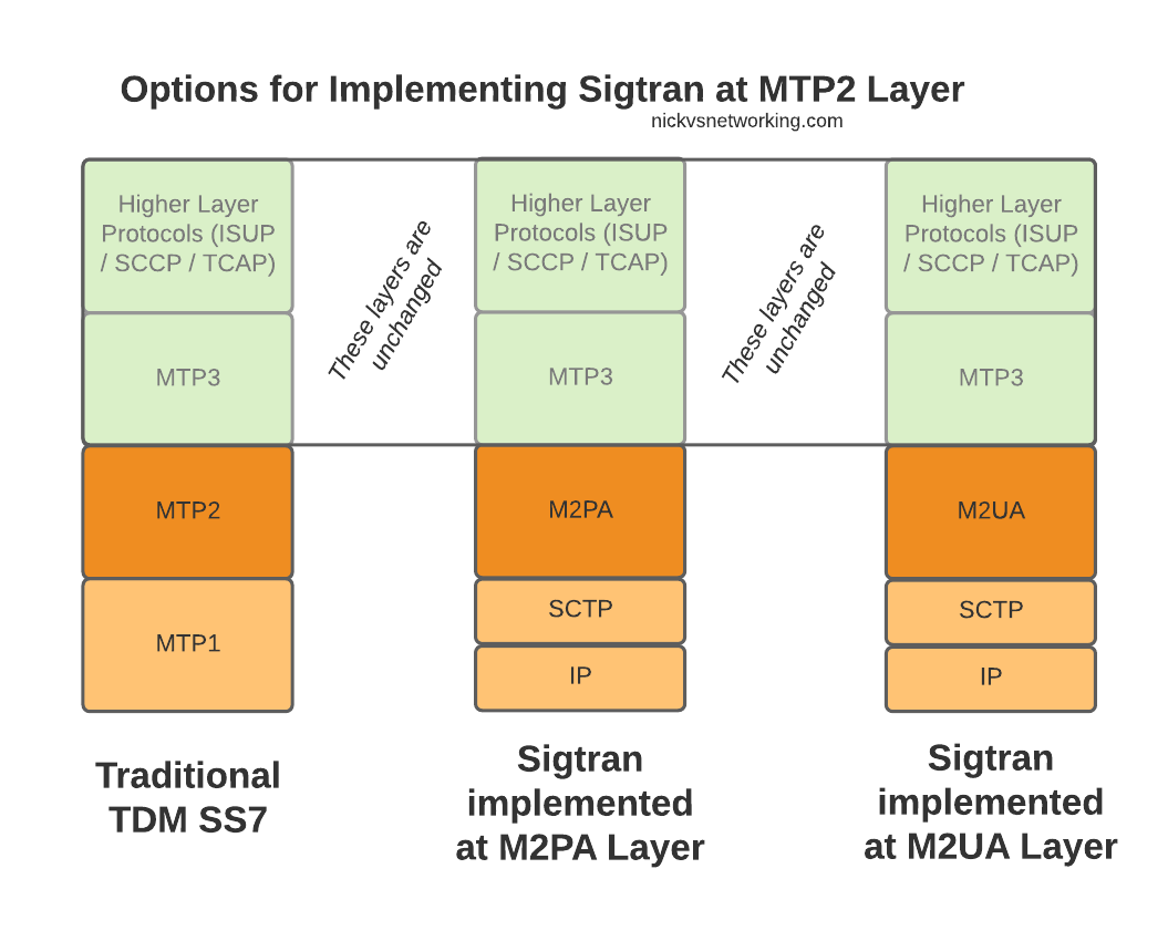
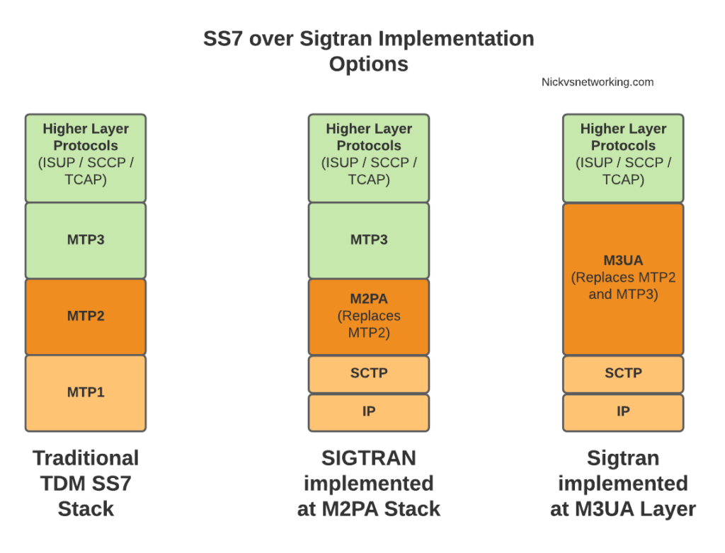
When we move from TDM based SS7 networks to IP based (Sigtran), MTP2 is removed, and can be replaced with one of two options for transporting Layer 2 messaging over IP, M2UA or M2PA.
All the layers above MTP2 on SS7 or M2UA/M2PA on Sigtran, are unchanged, and the upper layers have no visability that underneath, MTP2 has been replaced with M2UA or M2PA.
Taking MTP2 and putting it onto an IP based Layer 2 protocol is only one option for implementing Sigtran, there are others that we’ll look into as we go along, but with this variant the upper layers above Layer 2 (MTP3) remain changed.
Putting SS7 Data Link Layer (MTP2) onto IP
So the two options – M2UA and M2PA. Why do we have two options?
SS7 networks can be really complicated, and different operators may have different needs when converting these networks to IP.
To satisfy those requirements, there’s a bunch of different flavors of SS7 over IP (Sigtran) available to implement, so operators can select the one that meets their needs and use cases.
This means when we’re learning it, there’s a stack of different options to cover.
On the Layer 2 Level, let’s look at the two options we have in some more detail.
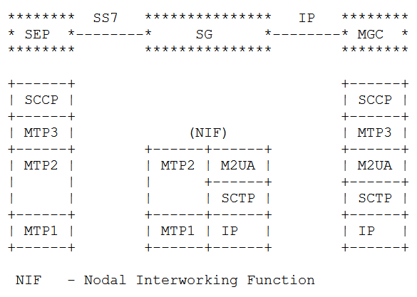
The M2UA Flavour
Image from RFC 4165 / 1.9. Differences Between M2PA and M2UA – Showing M2UA
With a “Nodal Interworking Function” using M2UA, the point codes between our two SS7 nodes remain unchanged.
The SS7 node on the left still talks MTP3 directly with the SS7 node on the right, and the NIF just transparently translates MTP2 into M2UA.
The best analogy I can come up with is that you can think of this as kind of like a Media Converter you’d use for converting between Cat5 to fibre – The devices at each end don’t know they’re not talking over a straight ethernet cable between them, but the media converter changes the transmission medium in between the two in a transparent manner.
M2UA acts in much the same way, except we’re transparently converting the layer 1 & layer 2 signaling, in a way that end devices in the network don’t need to be aware of.
The advantage of this option is that no config changes are needed, we’ve taken our Linksets that were running on TDM and converted them to IP so both ends of the linkset can be moved anywhere with IP connectivity, but transparently to the end devices.
For some carriers this is a real advantage – If you’ve got a dusty SSP running parts of your Customer Access Network, but the engineers who set it up retired long ago and you just want to drop those leased lines, M2UA could be a good option for you.
The disadvantage, as you might have guessed, is that we don’t get much value from just replacing the link from one point to another. It solves one problem, but doesn’t take that much of a step towards converging our network to run over IP.
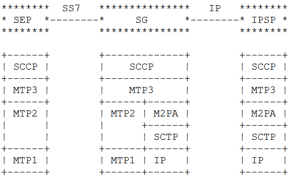
The M2PA Way
The M2PA way looks a bit different. You’ll notice we’ve got MTP3 on the Signaling Gateway we’re introducing into the network.
This means we need to add a point code between the SS7 node on the left and the SS7 node on the right, where there wasn’t one before, and we will need to update the routing tables on both to know to now route to each other via the point code of our Signaling Gateway rather than directly as the would have before we introduced the Signaling Gateway.
Image from RFC 4165 / 1.9. Differences Between M2PA and M2UA – Showing M2PA
We add another point code and an “active” SS7 device, but now we’ve got a lot more flexibility with what we can do, this no longer needs to be a point-to-point link, but with the introduction of the Signaling Gateway can be point-to-multipoint.
So which to chose? Well the answer is (as always) it depends.
If you cannot change any config on the end device (as the person who understood how all this stuff works retired long ago), then M2UA is the answer. M2UA is just an extension/branch of the MTP2 layer onto IP, it has no understanding / support for the higher-layers of SS7. M2UA is simpler, it doesn’t require as much understanding, it’s a quick-and-easy “drop-in” replacement for back-hauling SS7 onto IP. As it’s fairly dumb, M2UA can also allow us to split the load on a high traffic device across two or more SS7 nodes behind it, somewhat like a layer 2 load balancer, but this use case is pretty irrelevant these days.
M2PA on the other hand introduces a new Point Code (Operating on Layer 3 / MTP3) in between the two devices. This means we introduce a new point code in the path, so have to reconfigure the end devices, but affords us access to a lot of newer features. We can do all sorts of fancy things like routing of MTP3 messages, on the Signaling Gateway. This allows us to structure our network in new ways, rather than just doing what we were doing before but over IP.
Summary
When it comes to taking SS7 traffic and putting it onto IP at the Layer 2 level, we looked at the two most common options – M2PA and M2UA, and the pros and cons of each.
In our next post we’ll look at doing away with MTP2 layer entirely when we look at M3UA…
In iOS 15, Apple added support for iPhones to support SMS over IMS networks – SMSoIP. Previously iPhone users have been relying on CSFB / SMSoNAS (Using the SGs interface) to send SMS on 4G networks.
Getting this working recently led me to some issues that took me longer than I’d like to admit to work out the root cause of…
I was finding that when sending a Mobile Termianted SMS to an iPhone as a SIP MESSAGE, the iPhone would send back the 200 OK to confirm delivery, but it never showed up on the screen to the user.
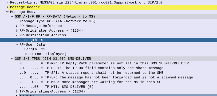
The GSM A-I/F headers in an SMS PDU are used primarily for indicating the sender of an SMS (Some carriers are configured to get this from the SIP From header, but the SMS PDU is most common).
The RP-Destination Address is used to indicate the destination for the SMS, and on all the models of handset I’ve been testing with, this is set to the MSISDN of the Subscriber.
But some devices are really finicky about it’s contents. Case in point, Apple iPhones.
If you send a Mobile Terminated SMS to an iPhone, like the one below, the iPhone will accept and send back a 200 OK to this request.
The problem is it will never be displayed to the user… The message is marked as delivered, the phone has accepted it it just hasn’t shown it…
SMS reports as delivered by the iPhone (200 OK back) but never gets displayed to the user of the phone as the RP-Destination Address header is populated
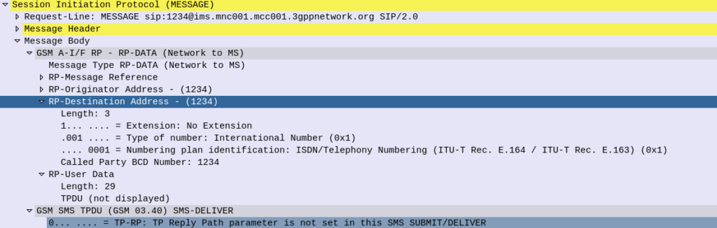
The fix is simple enough, if you set the RP-Destination Address header to 0, the message will be displayed to the user, but still took me a shamefully long time to work out the problem.
RP-Destination Address set to 0 sent to the iPhone, this time it’ll get displayed to the user.
I’ve become a big fan of Redis, and recently I had a need to integrate it into Kamailio.
There are two modules for integrating Kamailio and Redis, each have different functionalities:
db_redis is used when you want to use Redis in lieu of MySQL, PostGres, etc, as the database backend, this would be useful for services like usrloc. Not all queries / function calls are supported, but can be used as a drop-in replacement for a lot of modules that need database connectivity.
ndb_redis exposes Redis functions from the Kamailio config file, in a much more generic way. That’s what we’ll be looking at today.
The setup of the module is nice and simple, we load the module and then define the connection to the Redis server:
With the above we’ve created a connection to the Redis server at 127.0.0.2, and it’s called MyRedisServer.
You can define multiple connections to multiple Redis servers, just give each one a different name to reference.
Now if we want to write some data to Redis (SET) we can do it from within the dialplan with:
redis_cmd("MyRedisServer", "SET foo bar", "r");
We can then get this data back with:
#Get value of key "foo" from Redis
redis_cmd("MyRedisServer", "GET foo", "r");
#Set avp "foo_value" to output from Redis
$avp(foo_value) = $redis(r=>value);
#Print out value of avp "foo_value" to syslog
xlog("Value of foo is:  $avp(foo_value))
At the same time, we can view this data in Redis directly by running:
nick@oldfaithful:~$ redis-cli GET foo
Likewise we can set the value of keys and the keys themselves from AVPs from within Kamailio:
#Set the Redis Key to be the Received IP, with the value set to the value of the AVP "youravp"
redis_cmd("MyRedisServer", "SET $ct $avp(youravp)", "r");
All of the Redis functions are exposed through this mechanism, not just get and set, for example we can set the TTL so a record deletes after a set period of time:
#Set key with value of the received IP to expire after 120 seconds
redis_cmd("MyRedisServer", "EXPIRE $ct 120", "r");
I recently used Redis for a distributed flooding prevention mechanism, where the Subscriber’s received IP is used as the key in Redis and the value set to the number of failed auth attempts that subscriber has had, by using Redis we’re able to use the same mechanism across different platforms and easily administer it.
After getting AMR support in FreeSWITCH I set about creating an IMS Application Server for VoLTE / IMS networks using FreeSWITCH.
So in IMS what is an Application Server? Well, the answer is almost anything that’s not a CSCF.
An Application Server could handle your Voicemail, recorded announcements, a Conference Factory, or help interconnect with other systems (without using a BGCF).
I’ll be using mine as a simple bridge between my SIP network and the IMS core I’ve got for VoLTE, with FreeSWITCH transcoding between AMR to PCMA.
Setting up FreeSWITCH
You’ll need to setup FreeSWITCH as per your needs, so that’s however you want to use it.
This post won’t cover setting up FreeSWITCH, there’s plenty of good resources out there for that.
The only difference is when you install FreeSWITCH, you will want to compile with AMR Support, so that you can interact with mobile phones using the AMR codec, which I’ve documented how to do here.
Setting up your IMS
In order to get calls from the IMS to the Application Server, we need a way of routing the calls to the Application Server.
There are two standards-compliant ways to achieve this,
But this is a blunt instrument, after all, it’ll only ever be used at the start of the call, what if we want to send it to an AS because a destination can’t be reached and we want to play back a recorded announcement?
This is part of a series of posts looking into SS7 and Sigtran networks. We cover some basic theory and then get into the weeds with GNS3 based labs where we will build real SS7/Sigtran based networks and use them to carry traffic.
Having a direct Linkset from every Point Code to every other Point Code in an SS7 network isn’t practical, we need to rely on routing, so in this post we’ll cover routing between Point Codes on our STPs.
Let’s start in the IP world, imagine a router with a routing table that looks something like this:
Simple IP Routing Table
192.168.0.0/24 out 192.168.0.1 (Directly Attached)
172.16.8.0/22 via 192.168.0.3 - Static Route - (Priority 100)
172.16.0.0/16 via 192.168.0.2 - Static Route - (Priority 50)
10.98.22.1/32 via 192.168.0.3 - Static Route - (Priority 50)
We have an implicit route for the network we’re directly attached to (192.168.0.0/24), and then a series of static routes we configure. We’ve also got two routes to the 172.16.8.0/22 subnet, one is more specific with a higher priority (172.16.8.0/22 – Priority 100), while the other is less specific with a lower priority (172.16.0.0/16 – Priority 50). The higher priority route will take precedence.
This should look pretty familiar to you, but now we’re going to take a look at routing in SS7, and for that we’re going to be talking Variable Length Subnet Masking in detail you haven’t needed to think about since doing your CCNA years ago…
Why Masking is Important
A route to a single Point Code is called a “/14”, this is akin to a single IPv4 address being called a “/32”.
We could setup all our routing tables with static routes to each point code (/14), but with about 4,000 international point codes, this might be a challenge.
Instead, by using Masks, we can group together ranges of Point Codes and route those ranges through a particular STP.
This opens up the ability to achieve things like “Route all traffic to Point Codes to this Default Gateway STP”, or to say “Route all traffic to this region through this STP”.
Individually routing to a point code works well for small scale networking, but there’s power, flexibility and simplification that comes from grouping together ranges of point codes.
Information Overload about Point Codes
So far we’ve talked about point codes in the X.YYY.Z format, in our lab we setup point codes like 1.2.3.
This is not the only option however…
Variants of SS7 Point Codes
IPv4 addresses look the same regardless of where you are. From Algeria to Zimbabwe, IPv4 addresses look the same and route the same.
In SS7 networks that’s not the case – There are a lot of variants that define how a point code is structured, how long it is, etc. Common variants are ANSI, ITU-T (International & National variants), ETSI, Japan NTT, TTC & China.
The SS7 variant used must match on both ends of a link; this means an SS7 node speaking ETSI flavoured Point Codes can’t exchange messages with an ANSI flavoured Point Code.
Well, you can kinda translate from one variant to another, but requires some rewriting not unlike how NAT does it.
ITU International Variant
For the start of this series, we’ll be working with the ITU International variant / flavour of Point Code.
ITU International point codes are 14 bits long, and format is described as 3-8-3. The 3-8-3 form of Point code just means the 14 bit long point code is broken up into three sections, the first section is made up of the first 3 bits, the second section is made up of the next 8 bits then the remaining 3 bits in the last section, for a total of 14 bits.
So our 14 bit 3-8-3 Point Code looks like this in binary form:
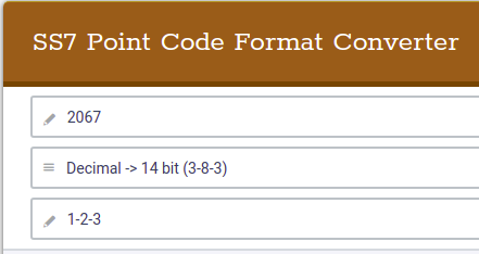
If you’re dealing with multiple vendors or products,you’ll see some SS7 Point Codes represented as decimal (2067), some showing as 1-2-3 codes and sometimes just raw binary. Fun hey?
So why does the binary part matter? Well the answer is for masks.
To loop back to the start of this post, we talked about IP routing using a network address and netmask, to represent a range of IP addresses. We can do the same for SS7 Point Codes, but that requires a teeny bit of working out.
As an example let’s imagine we need to setup a route to all point codes from 3-4-0 through to 3-6-7, without specifying all the individual point codes between them.
Firstly let’s look at our start and end point codes in binary:
100-00000100-000 = 3-004-0 (Start Point Code)
100-00000110-111 = 3-006-7 (End Point Code)
Looking at the above example let’s look at how many bits are common between the two,
100-00000100-000 = 3-004-0 (Start Point Code)
100-00000110-111 = 3-006-7 (End Point Code)
The first 9 bits are common, it’s only the last 5 bits that change, so we can group all these together by saying we have a /9 mask.
When it comes time to add a route, we can add a route to 3-4-0/9 and that tells our STP to match everything from point code 3-4-0 through to point code 3-6-7.
The STP doing the routing it only needs to match on the first 9 bits in the point code, to match this route.
SS7 Routing Tables
Now we have covered Masking for roues, we can start putting some routes into our network.
In order to get a message from one point code to another point code, where there isn’t a direct linkset between the two, we need to rely on routing, which is performed by our STPs.
This is where all that point code mask stuff we just covered comes in.
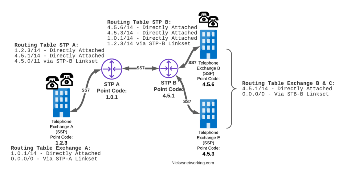
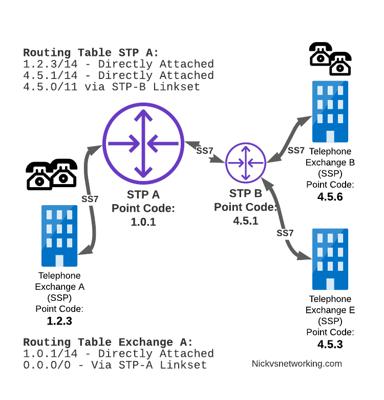
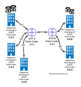
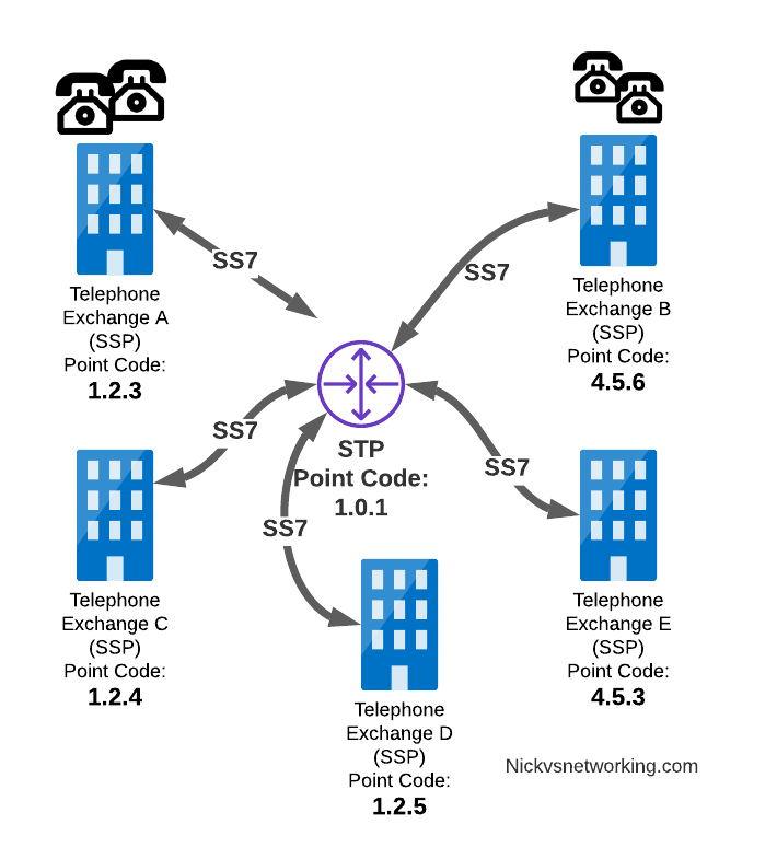
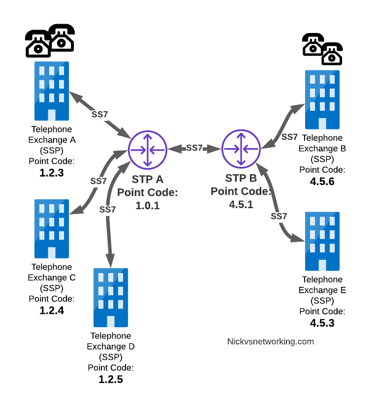
Let’s look at a diagram below,
Let’s look at the routing to get a message from Exchange A (SSP) on the bottom left of the picture to Exchange E (SSP) with Point Code 4.5.3 in the bottom right of the picture.
Exchange A (SSP) on the bottom left of the picture has point code 1.2.3 assigned to it and a Linkset to STP-A. It has the implicit route to STP-A as it’s got that linkset, but it’s also got a route configured on it to reach any other point code via the Linkset to STP-A via the 0.0.0/0 route which is the SS7 equivalent of a default route. This means any traffic to any point code will go to STP-A.
From STP-A we have a linkset to STP-B. In order to route to the point codes behind STP-B, STP-A has a route to match any Point Code starting with 4.5.X, which is 4.5.0/11. This means that STP-A will route any Point Code between 4.5.1 and 4.5.7 down the Linkset to STP-B.
STP-B has got a direct connection to Exchange B and Exchange E, so has implicit routes to reach each of them.
So with that routing table, Exchange A should be able to route a message to Exchange E.
But…
Return Routing
Just like in IP routing, we need return routing. while Exchange A (SSP) at 1.2.3 has a route to everywhere in the network, the other parts of the network don’t have a route to get to it. This means a request from 1.2.3 can get anywhere in the network, but it can’t get a response back to 1.2.3.
So to get traffic back to Exchange A (SSP) at 1.2.3, our two Exchanges on the right (Exchange B & C with point codes 4.5.6 and 4.5.3) will need routes added to them. We’ll also need to add routes to STP-B, and once we’ve done that, we should be able to get from Exchange A to any point code in this network.
There is a route missing here, see if you can pick up what it is!
So we’ve added a default route via STP-B on Exchange B & Exchange E, and added a route on STP-B to send anything to 1.2.3/14 via STP-A, and with that we should be able to route from any exchange to any other exchange.
One last point on terminology – when we specify a route we don’t talk in terms of the next hop Point Code, but the Linkset to route it down. For example the default route on Exchange A is 0.0.0/0 via STP-A linkset (The linkset from Exchange A to STP-A), we don’t specify the point code of STP-A, but just the name of the Linkset between them.
Back into the Lab
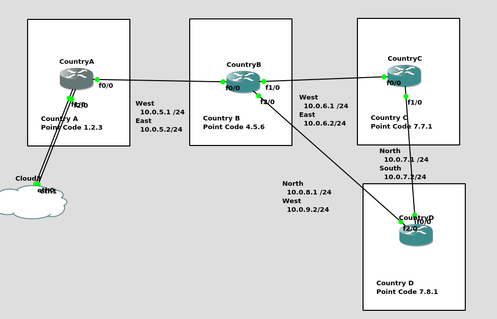
So back to the lab, where we left it was with linksets between each point code, so each Country could talk to it’s neighbor.
Let’s confirm this is the case before we go setting up routes, then together, we’ll get a route from Country A to Country C (and back).
So let’s check the status of the link from Country B to its two neighbors – Country A and Country C. All going well it should look like this, and if it doesn’t, then stop by my last post and check you’ve got everything setup.
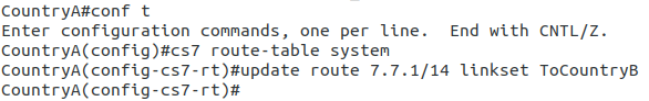
So let’s add some routing so Country A can reach Country C via Country B. On Country A STP we’ll need to add a static route. For this example we’ll add a route to 7.7.1/14 (Just Country C).
That means Country A knows how to get to Country C. But with no return routing, Country C doesn’t know how to get to Country A. So let’s fix that.
We’ll add a static route to Country C to send everything via Country B.
CountryC#conf t
Enter configuration commands, one per line.  End with CNTL/Z.
CountryC(config)#cs7 route-table system
CountryC(config)#update route 0.0.0/0 linkset ToCountryB
*Jan 01 05:37:28.879: %CS7MTP3-5-DESTSTATUS: Destination 0.0.0 is accessible
So now from Country C, let’s see if we can ping Country A (Ok, it’s not a “real” ICMP ping, it’s a link state check message, but the result is essentially the same).
By running:
CountryC# ping cs7 1.2.3
*Jan 01 06:28:53.699: %CS7PING-6-RTT: Test Q.755 1.2.3: MTP Traffic test rtt 48/48/48
*Jan 01 06:28:53.699: %CS7PING-6-STAT: Test Q.755 1.2.3: MTP Traffic test 100% successful packets(1/1)
*Jan 01 06:28:53.699: %CS7PING-6-RATES: Test Q.755 1.2.3: Receive rate(pps:kbps) 1:0 Sent rate(pps:kbps) 1:0
*Jan 01 06:28:53.699: %CS7PING-6-TERM: Test Q.755 1.2.3: MTP Traffic test terminated.
We can confirm now that Country C can reach Country A, we can do the same from Country A to confirm we can reach Country B.
But what about Country D? The route we added on Country A won’t cover Country D, and to get to Country D, again we go through Country B.
This means we could group Country C and Country D into one route entry on Country A that matches anything starting with 7-X-X,
For this we’d add a route on Country A, and then remove the original route;
Of course, you may have already picked up, we’ll need to add a return route to Country D, so that it has a default route pointing all traffic to STP-B. Once we’ve done that from Country A we should be able to reach all the other countries:
CountryA#show cs7 route
Dynamic Routes 0 of 1000

Routing table = system Destinations = 3 Routes = 3

Destination            Prio Linkset Name        Route
---------------------- ---- ------------------- -------
4.5.6/14         acces   1  ToCountryB          avail
7.0.0/3          acces   5  ToCountryB          avail


CountryA#ping cs7 7.8.1
*Jan 01 07:28:19.503: %CS7PING-6-RTT: Test Q.755 7.8.1: MTP Traffic test rtt 84/84/84
*Jan 01 07:28:19.503: %CS7PING-6-STAT: Test Q.755 7.8.1: MTP Traffic test 100% successful packets(1/1)
*Jan 01 07:28:19.503: %CS7PING-6-RATES: Test Q.755 7.8.1: Receive rate(pps:kbps) 1:0  Sent rate(pps:kbps) 1:0
*Jan 01 07:28:19.507: %CS7PING-6-TERM: Test Q.755 7.8.1: MTP Traffic test terminated.
CountryA#ping cs7 7.7.1
*Jan 01 07:28:26.839: %CS7PING-6-RTT: Test Q.755 7.7.1: MTP Traffic test rtt 60/60/60
*Jan 01 07:28:26.839: %CS7PING-6-STAT: Test Q.755 7.7.1: MTP Traffic test 100% successful packets(1/1)
*Jan 01 07:28:26.839: %CS7PING-6-RATES: Test Q.755 7.7.1: Receive rate(pps:kbps) 1:0  Sent rate(pps:kbps) 1:0
*Jan 01 07:28:26.843: %CS7PING-6-TERM: Test Q.755 7.7.1: MTP Traffic test terminated.
So where to from here?
Well, we now have a a functional SS7 network made up of STPs, with routing between them, but if we go back to our SS7 network overview diagram from before, you’ll notice there’s something missing from our lab network…
So far our network is made up only of STPs, that’s like building a network only out of routers!
In our next lab, we’ll start adding some SSPs to actually generate some SS7 traffic on the network, rather than just OAM traffic.
This is part of a series of posts looking into SS7 and Sigtran networks. We cover some basic theory and then get into the weeds with GNS3 based labs where we will build real SS7/Sigtran based networks and use them to carry traffic.
So we’ve made it through the first two parts of this series talking about how it all works, but now dear reader, we build an SS7 Lab!
At one point, and SS7 Signaling Transfer Point would be made up of at least 3 full size racks, and cost $5M USD. We can run a dozen of them inside GNS3!
Cisco’s “IP Transfer Point” (ITP) software adds SS7 STP functionality to some models of Cisco Router, like the 2651XM and C7200 series hardware.
Luckily for us, these hardware platforms can be emulated in GNS3, so that’s how we’ll be setting up our instances of Cisco’s ITP product to use as STPs in our network.
For the rest of this post series, I’ll refer to Cisco’s IP Transfer Point as the “Cisco STP”.
Not open source you say! Osmocom have OsmoSTP, which we’ll introduce in a future post, and elaborate on why later…
From inside GNS3, we’ll create a new template as per the Gif below.
You will need a copy of the software image to load in. If you’ve got software entitlements you should be able to download it, the filename of the image I’m using for the 7200 series is c7200-itpk9-mz.124-15.SW.bin and if you go searching, you should find it.
Now we can start building networks with our Cisco STPs!
What we’re going to achieve
In this lab we’re going to introduce the basics of setting up STPs using Sigtran (SS7 over IP).
If you follow along, by the end of this post you should have two STPs talking Sigtran based SS7 to each other, and be able to see the SS7 packets in Wireshark.
As we touched on in the last post, there’s a lot of different flavours and ways to implement SS7 over IP. For this post, we’re going to use M2PA (MTP2 Peer Adaptation Layer) to carry the MTP2 signaling, while MTP3 and higher will look the same as if it were on a TDM link. In a future post we’ll better detail the options here, the strengths and weaknesses of each method of transporting SS7 over IP, but that’s future us’ problem.
IP Connectivity
As we don’t have any TDM links, we’re going to do everything on IP, this means we have to setup the IP layer, before we can add any SS7/Sigtran stuff on top, so we’re going to need to get basic IP connectivity going between our Cisco STPs.
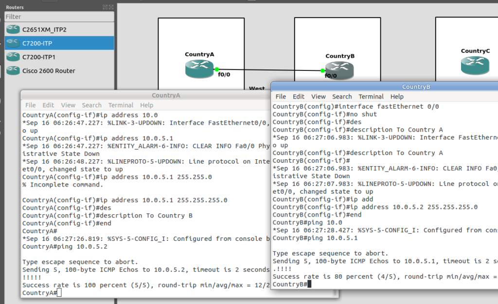
So for this we’ll need to set an IP Address on an interface, unshut it, link the two STPs. Once we’ve confirmed that we’ve got IP connectivity running between the two, we can get started on the Sigtran / SS7 side of things.
Let’s face it, if you’re reading this, I’m going to bet that you are probably aware of how to configure a router interface.
I’ve put a simple template down in the background to make a little more sense, which I’ve attached here if you want to follow along with the same addressing, etc.
So we’ll configure all the routers in each country with an IP – we don’t need to configure IP routing. This means adjacent countries with a direct connection between them should be able to ping each other, but separated countries shouldn’t be able to.
So now we’ve got IP connectivity between two countries, let’s get Sigtran / SS7 setup!
First we’ll need to define the basics, from configure-terminal in each of the Cisco STPs. We’ll need to set the SS7 variant (We’ll use ITU variant as we’re simulating international links), the network-indicator (This is an International network, so we’ll use that) and the point code for this STP (From the background image).
CountryA(config)#cs7 variant itu
CountryA(config)#cs7 network-indicator international
CountryA(config)#cs7 point-code 1.2.3
Repeat this step on Country A and Country B.
Next we’ll define a local peer on the STP. This is an instance of the Sigtran stack along with the port we’ll be listening on. Our remote peer will need to know this value to bring up the connection, the number specified is the port, and the IP is the IP it will bind on.
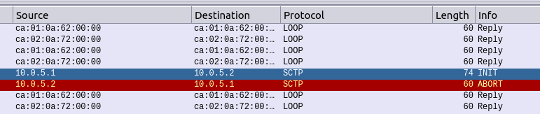
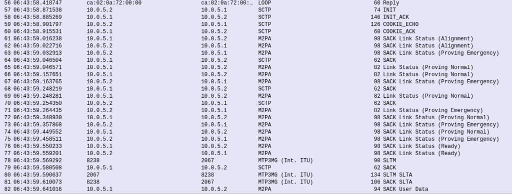
If you’re still sniffing the traffic between Country A and Country B, you should see our SS7 connection come up.
Wireshark trace of the connection coming up
The conneciton will come up layer-by-layer, firstly you’ll see the transport layer (SCTP) bring up an SCTP association, then MTP2 Peer Adaptation Layer (M2PA) will negotiate up to confirm both ends are working, then finally you’ll see MTP3 messaging.
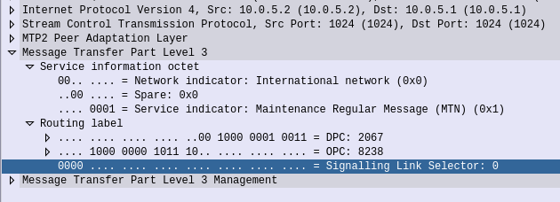
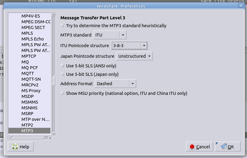
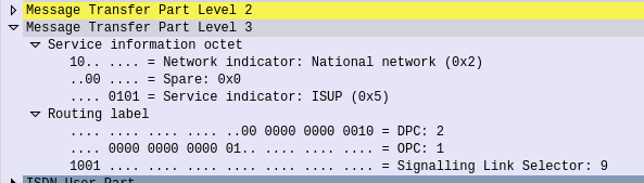
If we open up an MTP3 packet you can see our Originating and Destination Point Codes.
Notice in Wireshark the Point Codes don’t show up as 1-2-3, but rather 2067? That’s because they’re formatted as Decimal rather than 14 bit, this handy converter will translate them for you, or you can just change your preference in Wireshark’s decoders to use the matching ITU POint Code Structure.
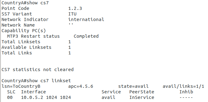
From the CLI on one of the two country STPs we can run some basic commands to view the status of all SS7 components and Linksets.
And there you have it! Basic SS7 connectivity!
There is so much more to learn, and so much more to do! By bringing up the link we’ve barely scratched the surface here.
Some homework before the next post, link all the other countries shown together, with Country D having a link to Country C and Country B. That’s where we’ll start in the lab – Tip: You’ll find you’ll need to configure a new cs7 local-peer for each interface, as each has its own IP.
This is part of a series of posts looking into SS7 and Sigtran networks. We cover some basic theory and then get into the weeds with GNS3 based labs where we will build real SS7/Sigtran based networks and use them to carry traffic.
So one more step before we actually start bringing up SS7 / Sigtran networks, and that’s to get a bit of a closer look at what components make up SS7 networks.
Recap: What is SS7?
SS7 is the name given to the protocol stack used almost exclusively in the telecommunications space. SS7 isn’t just one protocol, instead it is a suite of protocols. In the same way when someone talks about IP networking, they’re typically not just talking about the IP layer, but the whole stack from transport to application, when we talk about an SS7 network, we’re talking about the whole stack used to carry messages over SS7.
And what is SIGTRAN?
Sigtran is “Signaling Transport”. Historically SS7 was carried over TDM links (Like E1 lines).
As the internet took hold, the “Signaling Transport” working group was formed to put together the standards for carrying SS7 over IP, and the name stuck.
I’ve always thought if I were to become a Mexican Wrestler (which is quite unlikely), my stage name would be DSLAM, but SIGTRAN comes a close second.
Today when people talk about SIGTRAN, they mean “SS7 over IP”.
What is in an SS7 Network?
SS7 Networks only have 3 types of network elements:
Service Switching Points (SSP)
Service Transfer Points (STP)
Service Control Points (SCP)
Service Switching Points (SSP)
Service Switching Points (SSPs) are endpoints in the network. They’re the users of the connectivity, they use it to create and send meaningful messages over the SS7 network, and receive and process messages over the SS7 network.
Like a PC or server are IP endpoints on an IP Network, which send and receive messages over the network, an SSP uses the SS7 network to send and receive messages.
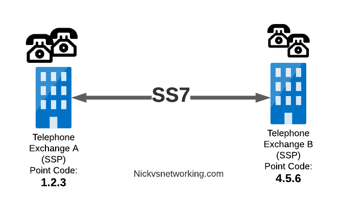
In a PSTN context, your local telephone exchange is most likely an SS7 Service Switching Point (SSP) as it creates traffic on the SS7 network and receives traffic from it.
A call from a user on one exchange to a user on another exchange could go from the SSP in Exchange A, to the SSP in Exchange B, in the same way you could send data between two computers by connecting directly between them with an Ethernet crossover cable.
Messages between our two exchanges are addressed using Point Codes, which can be thought of a lot like IP Addresses, except shorter.
In the MTP3 header of each SS7 message is the Destination Point Code, and the Origin Point Code.
When Telephone Exchange A wants to send a message over SS7 to Telephone Exchange B, the MTP header would look like:
MTP3 Header:
Origin Point Code:      1.2.3
Destination Point Code: 4.5.6
Service Transfer Points (STP)
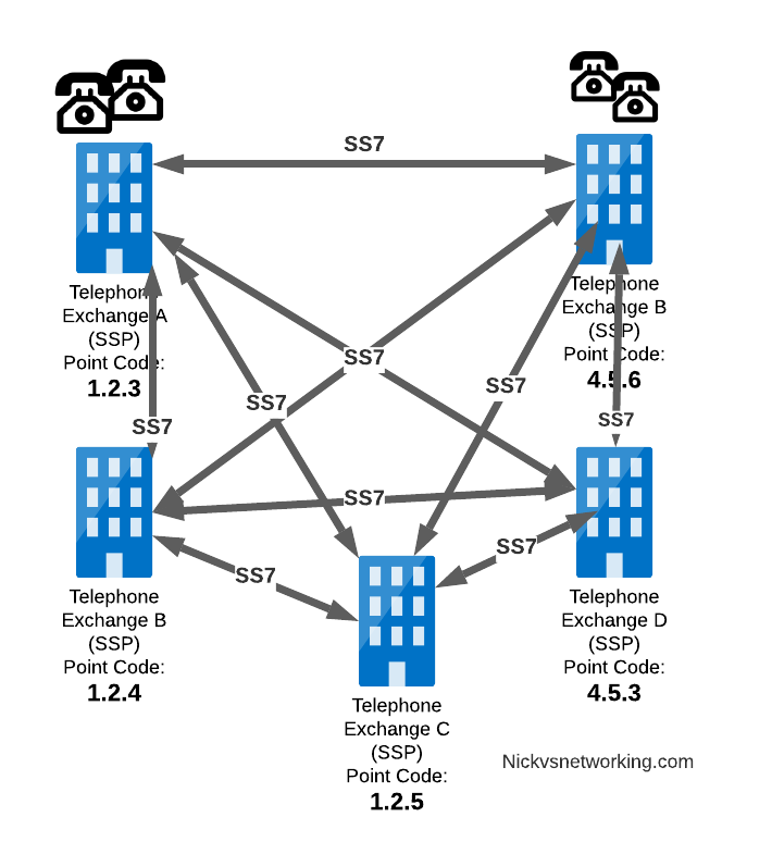
Linking each SSP to each other SSP has a pretty obvious problem as our network grows.
What happens if we’ve got hundreds of SSPs? If we want a full-mesh topology connecting every SSP to every other SSP directly, we’d have a rats nest of links!
A “full-mesh” approach for connecting SSPs does not work at scale, so STPs are introduced
So to keep things clean and scalable, we’ve got Signalling Transfer Points (STPs).
STPs can be thought of like Routers but in an SS7 network.
When our SSP generates an SS7 message, it’s typically handed to an STP which looks at the Destination Point Code, it’s own routing table and routes it off to where it needs to go.
STP acting as a central router to connect lots of SSPs
This means every SSP doesn’t require a connection to every other SSP. Instead by using STPs we can cut down on the complexity of our network.
When Telephone Exchange A wants to send a message over SS7 to Telephone Exchange B, the MTP header would look the same, but the routing table on Telephone Exchange A would be setup to send the requests out the link towards the STP.
MTP3 Header:
Origin Point Code:      1.2.3
Destination Point Code: 4.5.6
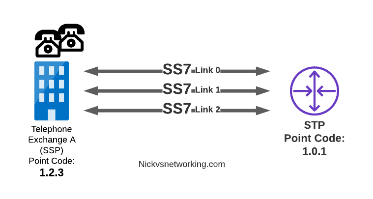
Linksets
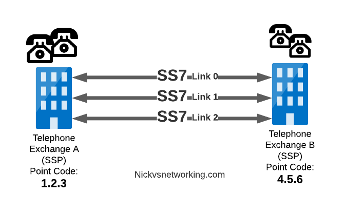
Between SS7 Nodes we have Linksets. Think of Linksets as like LACP or Etherchannel, but for SS7.
You want to have multiple links on every connection, for sharing out the load or for redundancy, and a Linkset is a group of connections from one SS7 node to another, that are logically treated as one link.
Link between an SSP and STP with 3 linksets
Each of the links in a Linkset is identified by a number, and specified in in the MTP3 header’s “Signaling Link Selector” field, so we know what link each message used.
MTP3 Header:
Origin Point Code:       1.2.3
Destination Point Code:  4.5.6
Signaling Link Selector: 2
Service Control Point (SCP)
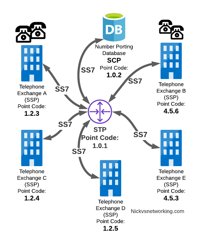
Somewhere between a Rolodex an relational database, is the Service Control Point (SCP).
For an exchange (SSP) to route a call to another exchange, it has to know the point code of the destination Exchange to send the call to. When fixed line networks were first deployed this was fairly straight forward, each exchange had a list of telephone number prefixes and the point code that served each prefix, simple.
But then services like number porting came along when a number could be moved anywhere. Then 1800/0800 numbers where a number had to be translated back to a standard phone number entered the picture.
To deal with this we need a database, somewhere an SSP can go to query some information in a database and get a response back.
This is where we use the Service Control Point (SCP).
Keep in mind that SS7 long predates APIs to easily lookup data from a service, so there was no RESTful option available in the 1980s.
When a caller on a local exchange calls a toll free (1800 or 0800 number depending on where you are) number, the exchange is setup with the Point Code of an SCP to query with the toll free number, and the SCP responds back with the local number to route the call to.
While SCPs are fading away in favor of technology like DNS/ENUM for Local Number Portability or Routing Databases, but they are still widely used in some networks.
Getting to know the Signalling Transfer Point (STP)
As we saw earlier, instead of a one-to-one connection between each SS7 device to every other SS7 device, Signaling Transfer Points (STP) are used, which act like routers for our SS7 traffic.
The STP has an internal routing table made up of the Point Codes it has connections to and some logic to know how to get to each of them.
Like a router, STPs don’t really create SS7 traffic, or consume traffic, they just receive SS7 messages and route them on towards their destination.
Ok, they do create some traffic for checking links are up, etc, but like a router, their main job is getting traffic where it needs to go.
When an STP receives an SS7 message, the STP looks at the MTP3 header. Specifically the Destination Point Code, and finds if it has a path to that Point Code. If it has a route, it forwards the SS7 message on to the next hop.
Like a router, an STP doesn’t really concern itself with anything higher than the MTP3 layer – As point codes are set in the MTP3 layer that’s the only layer the STP looks at and the upper layers aren’t really “any of its business”.
STPs don’t require a direct connection (Linkset) from the Originating Point Code straight to the Destination Point Code. Just like every IP router doesn’t need a direct connection to ever other network. By setting up a routing table of Point Codes and Linksets as the “next-hop”, we can reach Destination Point Codes we don’t have a direct Linkset to by routing between STPs to reach the final Destination Point Code.
Let’s work through an example:
And let’s look at the routing table setup on STP-A:
STP A Routing Table:
1.2.3 - Directly attached (Telephone Exchange A)
1.2.4 - Directly attached (Telephone Exchange C)
1.2.5 - Directly attached (Telephone Exchange D)
4.5.1 - Directly attached (STP-B)
4.5.3 - Via STP-B
4.5.6 - Via STP-B
So what happens when Telephone Exchange A (Point Code 1.2.3) wants to send a message to Telephone Exchange E (Point Code 4.5.3)? Firstly Telephone Exchange A puts it’s message on an MTP3 payload, and the MTP3 header will look something like this:
MTP3 Header:
Origin Point Code:       1.2.3
Destination Point Code:  4.5.3
Signaling Link Selector: 1
Telephone Exchange A sends the SS7 message to STP A, which looks at the MTP3 header’s Destination Point Code (4.5.3), and then in it’s routing table for a route to the destination point. We can see from our example routing table that STP A has a route to Destination Point Code 4.5.3 via STP-B, so sends it onto STP-B.
For STP-B it has a direct connection (linkset) to Telephone Exchange E (Point Code 4.5.3), so sends it straight on
Like IP, Point Codes have their own form of Variable-Length-Subnet-Routing which means each STP doesn’t need full routing info for every Destination Point Code, but instead can have routes based on part of the point code and a subnet mask.
But unlike IP, there is no BGP or OSPF on SS7 networks. Instead, all routes have to be manually specified.
For STP A to know it can get messages to destinations starting with 4.5.x via STP B, it needs to have this information manually added to it’s route table, and the same for the return routing.
Sigtran & SS7 Over IP
As the world moved towards IP enabled everything, TDM based Sigtran Networks became increasingly expensive to maintain and operate, so a IETF taskforce called SIGTRAN (Signaling Transport) was created to look at ways to move SS7 traffic to IP.
When moving SS7 onto IP, the first layer of SS7 (MTP1) was dropped, as it primarily concerned the physical side of the network. MTP2 didn’t really fit onto an IP model, so a two options were introduced for transport of the MTP2 data, M2PA (Message Transfer Part 2 User Peer-to-Peer Adaptation Layer) and M2UA (MTP2 User Adaptation Layer) were introduced, which rides on top of SCTP. This means if you wanted an MTP2 layer over IP, you could use M2UA or M2TP.
SCTP is neither TCP or UDP. I’ve touched upon SCTP on this blog before, it’s as if you took the best bits of TCP without the issues like head of line blocking and added multi-homing of connections.
So if you thought all the layers above MTP2 are just transferred, unchanged on top of our M2PA layer, that’s one way of doing it, however it’s not the only way of doing it.
There are quite a few ways to map SS7 onto IP Networks, which we’ll start to look into it more detail, but to keep it simple, for the next few posts we’ll be assuming that everything above MTP2/M2PA remain unchanged.
In the next post, we’ll get some actual SS7 traffic flowing!
This is part of a series of posts looking into SS7 and Sigtran networks. We cover some basic theory and then get into the weeds with GNS3 based labs where we will build real SS7/Sigtran based networks and use them to carry traffic.
If you use a mobile phone, a VoIP system or a copper POTS line, there’s a high chance that somewhere in the background, SS7 based signaling is being used.
The signaling for GSM, UMTS and WCDMA mobile networks all rely on SS7 based signaling, and even today the backbone of most PSTN traffic relies SS7 networks. To many this is mysterious carrier tech, and as such doesn’t get much attention, but throughout this series of posts we’ll take a hands-on approach to putting together an SS7 network using GNS3 based labs and connect devices through SS7 and make some stuff happen.
Overview of SS7
Signaling System No. 7 (SS7/C7) is the name for a family of protocols originally designed for signaling between telephone switches. In plain English, this means it was used to setup and teardown large volumes of calls, between exchanges or carriers.
When carrier A and Carrier B want to send calls between each other, there’s a good chance they’re doing it over an SS7 Network.
But wait! SIP exists and is very popular, why doesn’t everyone just use SIP? Good question, imaginary asker. The answer is that when SS7 came along, SIP was still almost 25 years away from being defined. Yes. It’s pretty old.
SS7 isn’t one protocol, but a family of protocols that all work together – A “protocol stack”. The SS7 specs define the lower layers and a choice of upper layer / application protocols that can be carried by them.
The layered architecture means that the application layer at the top can be changed, while the underlying layers are essentially the same.
This means while SS7’s original use was for setting up and tearing down phone calls, this is only one application for SS7 based networks. Today SS7 is used heavily in 2G/3G mobile networks for connectivity between core network elements in the circuit-switched domain, for international roaming between carriers and services like Local Number Portability and Toll Free numbers.
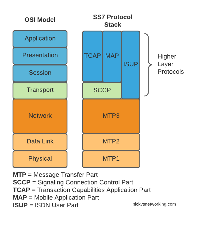
Here’s the layers of SS7 loosely mapped onto the OSI model (SS7 predates the OSI model as well):
OSI Model (Left) and SS7 Protocol Stack (Right)
We do have a few layers to play with here, and we’ll get into them all in depth as we go along, but a brief introduction to the underlying layers:
MTP 1 – Message Transfer Part 1
This is our physical layer. In this past this was commonly E1/T1 lines.
It’s responsible for getting our 1s and 0s from one place to another.
MTP 2 – Message Transfer Part 2
MTP2 is responsible for the data link layer, handling reliable transfer of data, in sequence.
MTP 3 – Message Transfer Part 3
The MTP3 header contains an Originating and a Destination Point Code.
These point codes can be thought of as like an IP Address; they’re used to address the source and destination of a message. A “Point Code” is the unique address of a SS7 Network element.
MTP3 header showing the Destination Point Code (DPC) and Origin Point Code (OPC) on a National Network, carrying ISUP traffic
Every message sent over an SS7 network will contain an Origin Point Code that identifies the sender, and a Destination Point Code that identifies the intended recipient.
This is where we’ll bash around at the start of this course, setting up Linksets to allow different devices talking to each other and addressing each other via Point Codes.
The MTP3 header also has a Service Indicator flag that indicates what the upper layer protocol it is carrying is, like the Protocol indicator in IPv4/IPv6 headers.
A Signaling Link Selector indicates which link it was transported over (did I mention we can join multiple links together?), and a Network Indicator for determining if this is signaling is at the National or International level.
TUP/MAP/SCCP/ISUP
These are the “higher-layer” protocols. Like FTP sits on top of TCP/IP, a SS7 network can transport these protocols from their source to their destination, as identified by the Origin Point Code (OPC), to the Destination Point Code (DPC), as specified in the MTP3 header.
We’ll touch on these protocols more as we go on. SCCP has it’s own addressing on top of the OPC/DPC (Like IP has IP Addressing, but TCP has port numbers on top to further differentiate).
Why learn SS7 today?
SS7 and SIGTRAN are still widely in use in the telco world, some of it directly, other parts derived / evolved from it.
So stick around, things are about to get interesting!
The SIP RFC allows for multiple SIP headers to have the same name,
For example, it’s very common to have lots of Via headers present in a request.
In Kamailio, we often may wish to add headers, view the contents of headers and perform an action or re-write headers (Disclaimer about not rewriting Vias as that goes beyond the purview of a SIP Proxy but whatever).
Let’s look at a use case where we have multiple instances of the X-NickTest: header, looking something like this:
INVITE sip:[email protected]:5061 SIP/2.0
X-NickTest: ENTRY ONE
X-NickTest: ENTRY TWO
X-NickTest: ENTRY THREE
...
Let’s look at how we’d access this inside Kamailio.
First, we could just use the psedovariable for header – $hdr()
xlog("Value of X-NickTest is: $hdr(X-NickTest)");
But this would just result in the first entry being printed out:
Value of X-NickTest is: ENTRY ONE
If we know how many instances there are of the header, we can access it by it’s id in the array, for example:
xlog("Value of first X-NickTest is: $hdr(X-NickTest)[0]");
xlog("Value of second X-NickTest is: $hdr(X-NickTest)[1]");
xlog("Value of third  X-NickTest is: $hdr(X-NickTest)[2]");
But we may not know how many to expect either, but we can find out using $hdrc(name) to get the number of headers returned.
xlog("X-NickTest has $hdrc(X-NickTest) entries");
You’re probably seeing where I’m going with this, the next logical step is to loop through them, which we can also do something like this:
$var(i) = 0;
while($var(i) < $hdrc(X-NickTest)) {
         xlog(X-NickTest entry [$var(i)] has value $hdrc(X-NickTest)[$var(i)]);
         $var(i) = $var(i) + 1;
}
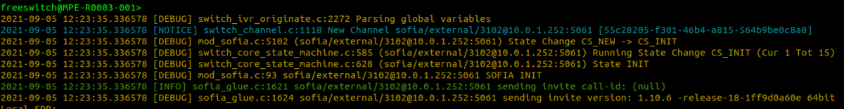
Through fs_cli you can orignate calls from FreeSWITCH.
At the CLI you can use the originate command to start a call, this can be used for everything from scheduled wake up calls, outbound call centers, to war dialing.
For example, what I’m using:
originate sofia/external/[email protected]:5061 61399999995 XML default
originate is the command on the FS_CLI
sofia/external/[email protected]:5061 is the call URL, with the application (I’m using mod_sofia, so sofia), the Sofia Profile (in my case external) and the SIP URI, or, if you have gateways configured, the to URI and the gateway to use.
6139999995 is the Application
XML is the Dialplan to reference
default is the Context to use
But running this on the CLI is only so useful, we can use an ESL socket to use software to connect to FreeSWITCH’s API (Through the same mechanism fs_cli uses) in order to programmatically start calls.
But to do that first we need to expose the ESL API for inbound connections (Clients connecting to FreeSWITCH’s ESL API, which is different to FreeSWITCH connecting to an external ESL Server where FreeSWITCH is the client).
We’ll need to edit the event_socket.conf.xml file to define how this can be accessed:
Obviously you’ll need to secure this appropriately, good long password, and tight ACLs.
You may notice after applying these changes in the config, you’re no longer able to run fs_cli and access FreeSWITCH, this is because FreeSWITCH’s fs_cli tool connects to FreeSWITCH over ESL, and we’ve just changed tha parameters. You should still be able to connect by specifying the IP Address, port and the secret password we set:
This also means we can run fs_cli from other hosts if permitted through the ACLs (kinda handy for managing larger clusters of FreeSWITCH instances).
But now we can also connect a remote ESL client to it to run commands like our Originate command to setup calls, I’m using GreenSwitch with ESL in Python:
import gevent
import greenswitch
import sys
#import Fonedex_TelephonyAPI
#sys.path.append('../WebUI/Flask/')
import uuid

import logging
logging.basicConfig(level=logging.DEBUG)


esl_server_host = "10.0.1.16"
logging.debug("Originating call to " + str(destination) + " from " + str(source))
logging.debug("Routing the call to " + str(dialplan_entry))
fs = greenswitch.InboundESL(host=str(esl_server_host), port=8021, password='yoursecretpassword')
  try:
      fs.connect()
      logging.debug("Connected to ESL server at " + str(esl_server_host))
  except:
      raise SystemError("Failed to connect to ESL Server at " + str(esl_server_host))

r = fs.send('bgapi originate {origination_caller_id_number=' + str(source) + '}sofia/external/' + str(destination) + '@10.0.1.252:5061 default XML')
Recently I was working on a project that required Kamailio to constantly re-evaluate something, and generate a UAC request if the condition was met.
There’s a few use cases for this: For example you might want to get Kamailio to constantly check the number of SIP registrations and send an alert if they drop below a certain number. If a subscriber drops out in that their Registration just expires, there’s no SIP message that will come in to tell us, so we’d never be able to trigger something in the normal Kamailio request_route.
Of you might want to continually send a SIP MESSAGE to pop up on someone’s phone to drive them crazy. That’s what this example will focus on.
This is where the rtimer module comes in. You can define the check in a routing block, and then
Early on as subscriber trunk dialing and automated time-based charging was introduced to phone networks, engineers were faced with a problem from Payphones.
Previously a call had been a fixed price, once the caller put in their coins, if they put in enough coins, they could dial and stay on the line as long as they wanted.
But as the length of calls began to be metered, it means if I put $3 of coins into the payphone, and make a call to a destination that costs $1 per minute, then I should only be allowed to have a 3 minute long phone call, and the call should be cutoff before the 4th minute, as I would have used all my available credit.
Conversely if I put $3 into the Payphone and only call a $1 per minute destination for 2 minutes, I should get $1 refunded at the end of my call.
We see the exact same problem with prepaid subscribers on IMS Networks, and it’s solved in much the same way.
In LTE/EPC Networks, Diameter is used for all our credit control, with all online charging based on the Ro interface. So let’s take a look at how this works and what goes on.
Generic 3GPP Online Charging Architecture
3GPP defines a generic 3GPP Online charging architecture, that’s used by IMS for Credit Control of prepaid subscribers, but also for prepaid metering of data usage, other volume based flows, as well as event-based charging like SMS and MMS.
Network functions that handle chargeable services (like the data transferred through a P-GW or calls through a S-CSCF) contain a Charging Trigger Function (CTF) (While reading the specifications, you may be left thinking that the Charging Trigger Function is a separate entity, but more often than not, the CTF is built into the network element as an interface).
The CTF is a Diameter application that generates requests to the Online Charging Function (OCF) to be granted resources for the session / call / data flow, the subscriber wants to use, prior to granting them the service.
So network elements that need to charge for services in realtime contain a Charging Trigger Function (CTF) which in turn talks to an Online Charging Function (OCF) which typically is part of an Online Charging System (AKA OCS).
For example when a subscriber turns on their phone and a GTP session is setup on the P-GW/PCEF, but before data is allowed to flow through it, a Diameter “Credit Control Request” is generated by the Charging Trigger Function (CTF) in the P-GW/PCEF, which is sent to our Online Charging Server (OCS).
The “Credit Control Answer” back from the OCS indicates the subscriber has the balance needed to use data services, and specifies how much data up and down the subscriber has been granted to use.
The P-GW/PCEF grants service to the subscriber for the specified amount of units, and the subscriber can start using data.
This is a simplified example – Decentralized vs Centralized Rating and Unit Determination enter into this, session reservation, etc.
The interface between our Charging Trigger Functions (CTF) and the Online Charging Functions (OCF), is the Ro interface, which is a Diameter based interface, and is common not just for online charging for data usage, IMS Credit Control, MMS, value added services, etc.
3GPP define a reference online-charging interface, the Ro interface, and all the application-specific interfaces, like the Gy for billing data usage, build on top of the Ro interface spec.
Basic Credit Control Request / Credit Control Answer Process
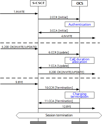
This example will look at a VoLTE call over IMS.
When a subscriber sends an INVITE, the Charging Trigger Function baked in our S-CSCF sends a Diameter “Credit Control Request” (CCR) to our Online Charging Function, with the type INITIAL, meaning this is the first CCR for this session.
The CCR contains the Service Information AVP. It’s this little AVP that is where the majority of the magic happens, as it defines what the service the subscriber is requesting. The main difference between the multitude of online charging interfaces in EPC networks, is just what the service the customer is requesting, and the specifics of that service.
For this example it’s a voice call, so this Service Information AVP contains a “IMS-Information” AVP. This AVP defines all the parameters for a IMS phone call to be online charged, for a voice call, this is the called-party, calling party, SDP (for differentiating between voice / video, etc.).
It’s the contents of this Service Information AVP the OCS uses to make decision on if service should be granted or not, and how many service units to be granted. (If Centralized Rating and Unit Determination is used, we’ll cover that in another post) The actual logic, relating to this decision is typically based on the the rating and tariffing, credit control profiles, etc, and is outside the scope of the interface, but in short, the OCS will make a yes/no decision about if the subscriber should be granted access to the particular service, and if yes, then how many minutes / Bytes / Events should be granted.
In the received Credit Control Answer is received back from our OCS, and the Granted-Service-Unit AVP is analysed by the S-CSCF. For a voice call, the service units will be time. This tells the S-CSCF how long the call can go on before the S-CSCF will need to send another Credit Control Request, for the purposes of this example we’ll imagine the returned value is 600 seconds / 10 minutes.
The S-CSCF will then grant service, the subscriber can start their voice call, and start the countdown of the time granted by the OCS.
As our chatty subscriber stays on their call, the S-CSCF approaches the limit of the Granted Service units from the OCS (Say 500 seconds used of the 600 seconds granted). Before this limit is reached the S-CSCF’s CTF function sends another Credit Control Request with the type UPDATE_REQUEST. This allows the OCS to analyse the remaining balance of the subscriber and policies to tell the S-CSCF how long the call can continue to proceed for in the form of granted service units returned in the Credit Control Answer, which for our example can be 300 seconds.
Eventually, and before the second lot of granted units runs out, our subscriber ends the call, for a total talk time of 700 seconds.
But wait, the subscriber been granted 600 seconds for our INITIAL request, and a further 300 seconds in our UPDATE_REQUEST, for a total of 900 seconds, but the subscriber only used 700 seconds?
The S-CSCF sends a final Credit Control Request, this time with type TERMINATION_REQUEST and lets the OCS know via the Used-Service-Unit AVP, how many units the subscriber actually used (700 seconds), meaning the OCS will refund the balance for the gap of 200 seconds the subscriber didn’t use.
If this were the interface for online charging of data, we’d have the PS-Information AVP, or for online charging of SMS we’d have the SMS-Information, and so on.
The architecture and framework for how the charging works doesn’t change between a voice call, data traffic or messaging, just the particulars for the type of service we need to bill, as defined in the Service Information AVP, and the OCS making a decision on that based on if the subscriber should be granted service, and if yes, how many units of whatever type.
The mod_httapi in FreeSWITCH allows you to upload your call recordings to a HTTP server, in my case I’ve put together a Flask based Python server for a project I’m working on, which when the call ends, uploads to my web server. Presto!
Obviously you’ll need to replace the URL etc, but you can then just extract the POSTed file out and boom, you don’t need to store any recordings on each FreeSWITCH instance.
This is fantastic if you’re running multiple instances in a cluster or containerized, and want every FreeSWITCH instance to be dumb and with access to the same data as every other instance.
So once we’ve got an ENUM server configured and confirmed we can query it and get the results we want using Dig, we can configure Kamailio.
But before we get to the Kamailio side, a word on how Kamailio handles DNS, Kamailio doesn’t have the ability to set a DNS server, instead it uses the system DNS server details, This means your system will need to use the DNS server we want to query for ENUM for all DNS traffic, not just for Kamailio. This means you may need to setup Recursion to still be able to query DNS records for the outside world.
To add support to Kamailio, we’ll need to load the enum module (enum.so),
In terms of parameters, all we’ll set is the doman_suffix, which is, as it sounds, the domain suffix used in the DNS queries. If you’re using a different domain for your ENUM it’d need to be reflected here.
modparam("enum", "domain_suffix", "e164.arpa.")
Next up inside our minimalist dialplan we’ll just add enum_query(); to query the SIP URI,
if(is_method("INVITE")){
         enum_query();
         xlog("Ran ENUM query");
         xlog("To URI $tU");
         forward();
}
Obviously in production you’d want to add more sanity checks and error handling, but with this, sending a SIP INVITE to Kamailio with an E.164 number in the SIP URI user part, will lead to an ENUM query resolving this, and routing the traffic to it,
In the last we covered what ENUM is and how it works, so to take this into a more practical example, I thought I’d share the details of the ENUM server I’ve setup in my lab, and the Docker container I’ve bundled it into.
Inside the Docker container we’ll be running Bind – this post won’t teach you much about Bind, there’s already lots of good information on it elsewhere, but we will cover the parameters involved in setting up ENUM records (NAPTR) for E.164 addresses.
Getting the Environment up and Running
First we’ll need to setup our environment, I’ve published the images for the container to Dockerhub, but we’ll build it from the Dockerfile so you can edit the files and rebuild as you play around:
systemd-resolve on Ubuntu binds to port 53 by default, which can lead to some headaches, so we’ll create a new network in Docker for this to run in, so it doesn’t conflict with anything else you may be running:
And now we’ll run the ENUM container in the enum_playground network and with the IP 172.30.0.2,
docker run -d --rm --name=enum --net=enum_playground --ip=172.30.0.2 enum
Ok, that’s the environment setup, let’s run some queries!
E.164 to SIP URI Resolution with ENUM
In our last post we covered the basics of formatting an E.164 number and querying a DNS server to get it’s call routing information.
Again we’re going to use Dig to query this information. In reality ENUM queries would be run by an endpoint, or software like FreeSWITCH or Kamailio (Spoiler alert, posts on ENUM handling in those coming later), but as we’re just playing Dig will work fine.
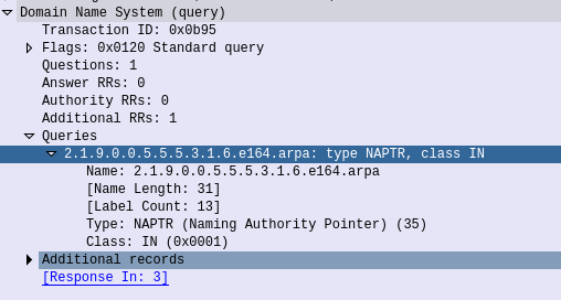
So let’s start by querying a single E.164 address, +61355500911
First we’ll reverse it and put full stops / periods between the numbers, to get 1.1.9.0.0.5.5.5.3.1.6
Next we’ll add the e164.arpa prefix, which is the global prefix for ENUM addresses, and presto, that’s what we’ll query – 1.1.9.0.0.5.5.5.3.1.6.e164.arpa
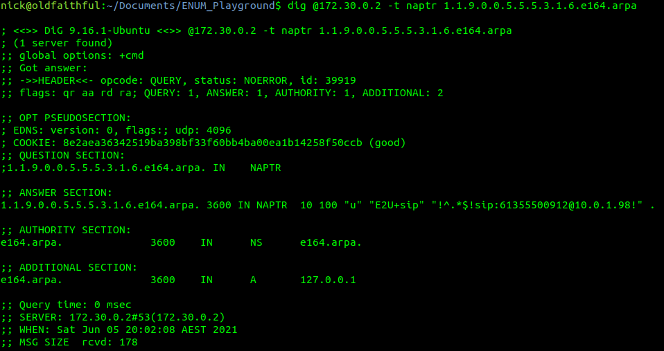
Lastly we’ll feed this into a Dig query against the IP of our container and of type NAPTR,
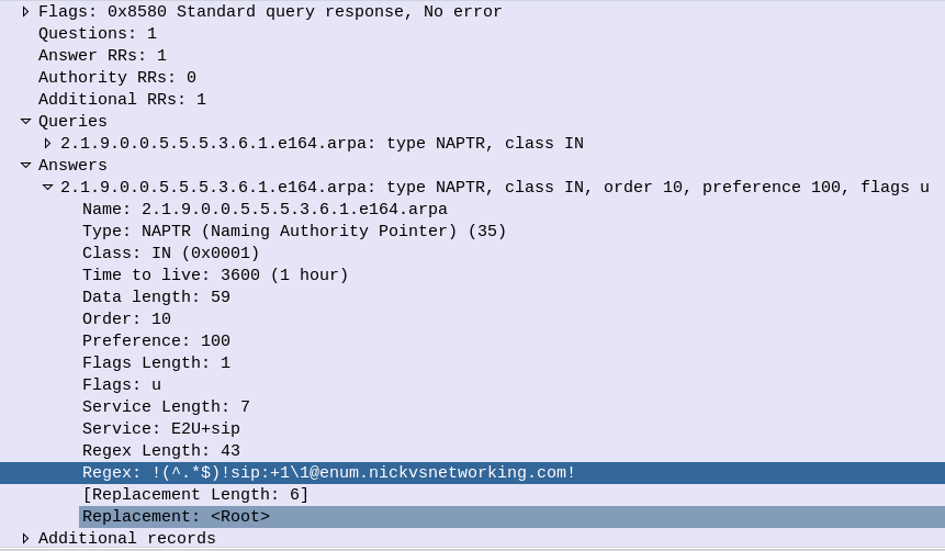
Next up is the TTL or expiry, in this case it’s 3600 seconds (1 hour), shorter periods allow for changes to propagate / be reflected more quickly but at the expense of more load as results can’t be cached for as long. The class (IN) represents Internet, which is the only class commonly used, even on internal systems.
Then we have the type of record returned, in our case it’s a NAPTR record,
1.1.9.0.0.5.5.5.3.1.6.e164.arpa.3600 IN NAPTR 10 100 "u" "E2U+sip" "!^.*$!sip:[email protected]!" .
After that is the Order, this defines the order in which the rules are to be parsed. Lower numbers are processed first, if no matches then the next lowest, and so on until the highest number is reached, we’ll touch on this in more detail later in this post,
1.1.9.0.0.5.5.5.3.1.6.e164.arpa.3600 IN NAPTR 10 100 "u" "E2U+sip" "!^.*$!sip:[email protected]!" .
The Pref is the processing preference. This is very handy for load balancing, as we can split traffic between hosts with different preferences. We’ll cover this later in this post too.
1.1.9.0.0.5.5.5.3.1.6.e164.arpa.3600 IN NAPTR 10 100 "u" "E2U+sip" "!^.*$!sip:[email protected]!" .
The Flags represent the type of record we’re going to get, for most ENUM traffic this is going to be set to U, to denote a SIP URI with Regex, while the Service value we’ll be looking for will be “E2U+sip” service to identify SIP URIs to route calls to, but could be other values like Email addresses, IM Addresses or PSTN numbers, to be parsed by other applications.
1.1.9.0.0.5.5.5.3.1.6.e164.arpa.3600 IN NAPTR 10 100 "u" "E2U+sip" "!^.*$!sip:[email protected]!" .
Lastly we’ve got the Regex part. Again not going to cover Regex as a whole, just the DNS particulars.
Everything between the first and second ! denotes what we’re searching for, while everything from the second ! to the last ! denotes what we replace it with.
In the below example that means we’re matching ^.* which means starting with (^) any character (.) zero or more times (*), which gets replaced with sip:[email protected],
1.1.9.0.0.5.5.5.3.1.6.e164.arpa.3600 IN NAPTR 10 100"u" "E2U+sip" "!^.*$!sip:[email protected]!" .
How should this be treated?
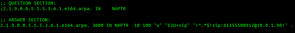
For the first example, a call to the E.164 address of 61355500912 will be first formatted into a domain as per the ENUM requirements (1.1.9.0.0.5.5.5.3.1.6.e164.arpa) and then queried as a NAPTR record against the DNS server,
1.1.9.0.0.5.5.5.3.1.6.e164.arpa.3600 IN NAPTR 10 100"u" "E2U+sip" "!^.*$!sip:[email protected]!" .
Only a single record has been returned so we don’t need to worry about the Order or Preference, and the Regex matches anything and replaces it with the resulting SIP URI of sip:[email protected], which is where we’ll send our INVITE.
Under the Hood
Inside the Repo we cloned earlier, if you open the e164.arpa.db file, things will look somewhat familiar,
The record we just queried is the first example in the Bind config file,
; E.164 Address +61355500911 - Simple no replacement (Resolves all traffic to sip:[email protected])
1.1.9.0.0.5.5.5.3.1.6 IN NAPTR 10 100 "u" "E2U+sip" "!^.*$!sip:[email protected]!" .
The config file is just the domain, class, type, order, preference, flags, service and regex.
Astute readers may have noticed the trailing . which where we can put a replacement domain if Regex is not used, but it cannot be used in conjunction with Regex, so for all our work it’ll just be a single trailing . on each line.
You can (and probably should) change the values in the e164.arpa.db file as we go along to try everything out, you’ll just need to rebuild the container and restart it each time you make a change.
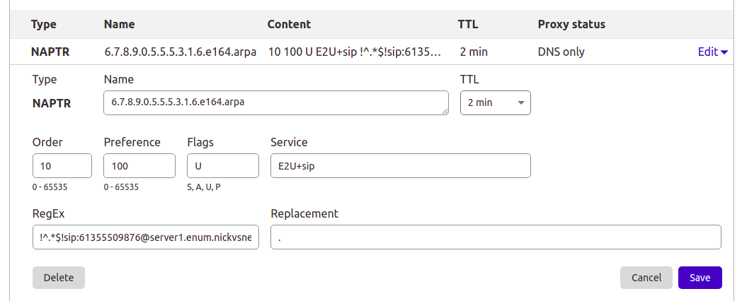
This post is going to focus on Bind, but the majority of modern DNS servers support NAPTR records, so you can use them for ENUM as well, for example I manage the DNS for this site thorough Cloudflare, and I’ve put a screenshot below of an example private ENUM address I’ve added into it.
Setting up a NAPTR record in Cloudflare DNS
Preference to Split Traffic between Servers
So with a firm understanding of a single record being returned, let’s look at how we can use ENUM to cleverly route traffic to multiple hosts.
If we have a pool of servers we may wish to evenly distribute all traffic across them, so that’s how E.164 address +61355500912 is setup – to route traffic evenly (50/50) across two servers.
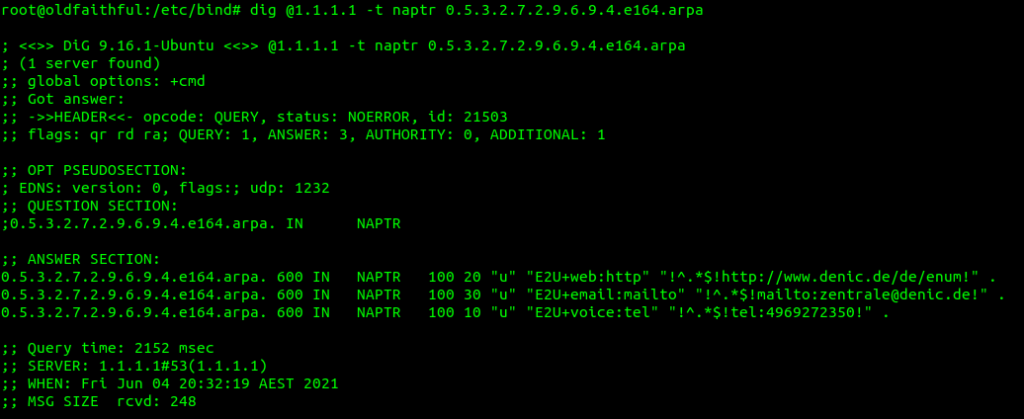
Querying it with Dig provides the following result:
So as the order value (10) is the same for both records, we can ignore it – there isn’t one value lower than the other.
We can see both records have a preference of 100, in practice, this means they each get 50% of the traffic. The formula for traffic distribution is pretty simple, each server gets the value of it’s preference, divided by the total of all the preferences,
So for server1 it’s preference is 100 and the total of all the preferences combined is 200, so it gets 100/200, which is equivalent to one half aka 50%.
We might have a scenario where we have 3 servers, but one is significantly more powerful than the others, so let’s look at giving more traffic to one server and less to others, this example gets a little more complex but should cement your understanding of how the preference works;
So now 3 servers, again none have a lower order than the other, it’s set to 10 for them all so we can ignore the order,
Next we can see the total of all the priority values is 400,
Server 2 has a priority of 100 so it gets 100/400 total priority, or a quarter of all traffic. Server 1 has the same value, so also gets a quarter of all traffic,
Server 3 however has a priority of 200 so it gets 200/400, or to simplify half of all traffic.
The Bind config for this is:
; E.164 Address +61355500913 - More complex load balance between 3 hosts (25% server1, 25% server2, 50% server3)
3.1.9.0.0.5.5.5.3.1.6 IN NAPTR 10 100 "u" "E2U+sip" "!^.*$!sip:[email protected]!" . 3.1.9.0.0.5.5.5.3.1.6 IN NAPTR 10 100 "u" "E2U+sip" "!^.*$!sip:[email protected]!" .
3.1.9.0.0.5.5.5.3.1.6 IN NAPTR 10 200 "u" "E2U+sip" "!^.*$!sip:[email protected]!" .
Order for Failover
Primarily the purpose of the order is to enable wildcard routes (as we’ll see later) to be overwritten by more specific routes, but a secondary use in some implementations use Order as a way to list the preferences of the SIP URIs to route to. For example we could have two servers, one a primary and the other a standby, with the standby only to be used only if the primary SIP URI was not responding.
E.164 number +61355500914 is setup to return two SIP URIs,
Our DNS client will first use the SIP URI sip:[email protected] as it has the lower order value (10), and if that fails, can try the entry with the next lowest order-value (20) which would be sip:[email protected].
The Bind config for this is:
; E.164 Address +61355500914 - Order example returning multiple SIP URIs to try for failover
4.1.9.0.0.5.5.5.3.1.6 IN NAPTR 10 100 "u" "E2U+sip" "!^.*$!sip:[email protected]!" . 4.1.9.0.0.5.5.5.3.1.6 IN NAPTR 20 100 "u" "E2U+sip" "!^.*$!sip:[email protected]!" .
Wildcards
If we have a 1,000 number block, having to add 1000 individual records can be very tedious. Instead we can use wildcard matching (thanks to the fact we’ve reversed the E.164 address) to match ranges. For example if we have E.164 numbers from +61255501000 to +61255501999 we can add a wildcard entry to match the +61255501x prefix,
I’ve set this up already so let’s lookup the E.164 number +6125501234,
If you look up any other number starting with +6125501 you’ll get the same result, and here’s the Bind config for it:
; Wildcard E.164 Address +61255501* - Wildcard example for all destinations starting with E.164 prefix +61255501x to single destination (sip:[email protected])
; For example E.164 number +6125501234 will resolve to sip:[email protected]
*.1.0.5.5.5.2.1.6 IN NAPTR 100 100 "u" "E2U+sip" "!^.*$!sip:[email protected]!" .
The catch with this is they’re all pointing at the same SIP URI, so we can’t treat the calls differently based on the called number – This is where the Regex magic comes in.
We can use group matching to match a group and fill it in the dialed number into the SIP Request URI, for example:
Will match the E.164 number requested and put it inside sip:[email protected]
The +61255502xxx prefix is setup for this, so if we query +61255502000 (or any other number between +61255502000 and +61255502999) we’ll get the regex query in the resulting record.
Keep in mind DNS doesn’t actually apply the Regex transformation, just shares it, and the client applies the transformation.
; Wildcard example for all destinations starting with E.164 prefix +61255502x to regex filled destination
; For example a request to 61255502000 will return sip:[email protected])
*.2.0.5.5.5.2.1.6 IN NAPTR 100 100 "u" "E2U+sip" "!(^.*$)!sip:+1\\[email protected]!" .
One last thing to keep in mind, is that Wildcard priorities are of any length. This means +612555021 would match as well as +6125550299999999999999. Typically terminating switches drop any superfluous digits, and NU those that are too short, but keep this in mind, that length is not taken into account.
Wildcard Priorities
So with our wildcards in place, what if we wanted to add an exception, for example one number in our 61255502xxx block of numbers gets ported to another carrier and needs to be routed elsewhere?
Easy, we just add another entry for that number being more specific and with a lower order than the wildcard, which is what’s setup for E.164 number +61255502345,
Which does not return the same result as the others that match the wildcard,
Bind config:
; Wildcard example for all destinations starting with E.164 prefix +61255502x to regex filled destination
; For example a request to +61255502000 will return sip:[email protected])
*.2.0.5.5.5.2.1.6 IN NAPTR 100 100 "u" "E2U+sip" "!(^.*$)!sip:+1\\[email protected]!" .

; More specific example with lower order than +6125550x wildcard for E.164 address +61255502345 will return sip:[email protected]
5.4.3.2.0.5.5.5.2.1.6 IN NAPTR 50 100 "u" "E2U+sip" "!^.*$!sip:[email protected]!" .
We can combine all of the tricks we’ve covered here, from statically defined entries, wildcards, regex replacement, multiple entries with multiple orders and preferences, to create really complex routing, using only DNS.
Summary & Next Steps
So by now hopefully you’ve got a fair understanding of how NAPTR and DNS work together to translate E.164 addresses into SIP URIs,
Of course being able to do this manually with Dig and comprehend how it’ll route is only one part of the picture, in the next posts we’ll cover using Kamailio and FreeSWITCH to query ENUM routing information and route traffic to it,
DNS is commonly used for resolving domain names to IP Addresses, and is often described as being like “the phone book of the Internet”.
So what’s the phone book of phone books?
The answer, is (kind of) DNS. With the aid of E.164 number to URI mapping (ENUM), DNS can be used to resolve phone numbers into SIP URIs to route the traffic to.
So what is ENUM?
ENUM allows us to bypass the need for a central switch for routing calls to numbers, and instead, through a DNS lookup, resolve a phone number into a reachable SIP URI that is the ultimate destination for the traffic.
Imagine you want to call a company, you dial the phone number for that company, your phone does a DNS query against the phone number, which returns the SIP URI of the company’s PBX, and your phone sends the SIP INVITE directly to the company’s PBX, with no intermediary party carrying the call.
3GPP have specified ENUM as the prefered mechanism for resolving phone numbers into SIP addresses, and while it’s widespread adoption on the public Internet is still in its early days (See my post on The Sad story of ENUM in Australia) it is increasingly common in IMS networks and inside operator networks.
ENUM allow us to lookup a phone number on a DNS server and find the SIP URI a server that will handle traffic for the phone number, but it’s a bit more complicated than the A or AAAA records you’d use to resolve a website, ENUM relies on NAPTR records.
Let’s look at the steps involved in taking an E.164 number and knowing where to send it.
Step 1 – Reverse the Numbers
We read phone numbers from left to right.
This is because historically the switch needs to get all the long-distance routing sorted first. The switch has to route your call to the exchange that serves that subscriber, which is what all the area codes and prefixes assigned to areas are all about (Throwback to SZU for any old Telco buffs).
For an E.164 number you’ve got a Country Code, Area Code and then the Subscriber Number. The number gets more specific as it goes along.
But getting more specific as you go along is the opposite how how DNS works, millions of domains share the .com suffix, and the unique / specific part is the bits before that.
So the first step in the ENUM process is to reverse the phone number, so let’s take phone number (03) 5550 0912, which in E.164 is +61 3 5550 0912.
As the spaces in the phone numbers are there for the humans, we’ll drop all of them and reverse the number, as DNS is more specific right-to-left, so we end up with
2.1.9.0.0.5.5.5.3.1.6
Step 2 – Add the Suffix
The ITU ENUM specifies the suffix e164.arpa be assigned for public ENUM entries. Private ENUM deployments may use their own suffix, but to make life simple I’m going to use e164.arpa as if it were public.
So we’ll append the e164.arpa domain onto our reversed and formatted E.164 phone number:
2.1.9.0.0.5.5.5.3.1.6.e164.arpa
Step 3 – Query it
Next we’ll run a Naming Authority Pointer (NAPTR) query against the domain, to get back a list of records for that number.
DNS is a big topic, and NAPTR and SRV takes up a good chunk of it, but what you need to know is that by using NAPTR we’re not limited to just a single response, we could have a weighted pool of servers handling traffic for this phone number, and be able to control load through the use of NAPTR, amongst other things.
DNS NAPTR QueryDNS NAPTR Response
Of course, if our phone can query the public NAPTR records, then so can anyone else, so we can just use a tool like Dig to query the record ourselves,
In the answers section I’ve setup this DNS server to only return a single response, with the regex SIP URI to use, in my case that’s sip:[email protected]
You’ll obviously need to replace the DNS server with your DNS server, and the query with the reversed and formatted version of the E.164 number you wish to query.
Step 4 – Send SIP traffic
After looking at the NAPTR records returned and using the weight and priority to determine which server/s to send to first, our phone forwards an INVITE to the URI returned in the NAPTR record.
How to interpret the returned results?
The first thing to keep in mind when working with ENUM is multiple records being returned is supported, and even encouraged.
NAPTR results return 7 fields, which define how it should be handled.
The host part is fairly obvious, and defines the host / DNS entry we’re talking about.
The Service defines what type of service this is. ENUM can be expanded beyond just voice, for example you may want to also return an email address or IM address as well as a SIP Address on an ENUM query, which you can do. By default voice uses the “E2U+sip” service to identify SIP URIs to route calls to, so in this context that’s what we’re interested in, but keep in mind there are other types out there,
Example ENUM query against a phone number showing other types of services (Email & Web)
The Order simply defines the order in which the rules are to be parsed. Lower numbers are processed first, if no matches then the next lowest, and so on until the highest number is reached.
The Pref is the processing preference. For load balancing 50/50 between two sites say a Melbourne and Sydney site, we’d return two results, with the same Order, and the same Pref, would see traffic split 50/50 between the two sites. We could split this further, a Pref value of 10 for Melbourne, 10 for Sydney, 5 for Brisbane and 5 for Perth would see 33% of calls route to Melbourne, 33% of calls route to Sydney, 16.5% of calls route to Brisbane and 16.5% of calls route to Perth. This is because we’d have a total preference value of 30, and the individual preference for each entry would work out as the fraction of the total (ie Pref 10 out of 30 = 10/30 or 33.3%).
The Flags denote the type of record we’re going to get, for most ENUM traffic this is going to be set to U, to denote a SIP URI with Regex.
The regexp field contains our SIP URI in the form of a Regular expression, which can include pattern matching and replacement. This is most commonly used to fill in the phone number into the SIP URI, for example instead of hardcoding the phone number into the response, we could use a Regular expression to fill in the requested number into the SIP URI.
If you’re looking to implement ENUM for an internal network, great, I’ll have some more posts here over the next few weeks covering off configuration of a DNS server to support ENUM lookups, and using Kamailio to lookup ENUM routes.
In terms of public ENUM, while many carriers are using ENUM inside their networks, public adoption of ENUM in most markets has been slow, for a number of reasons.
Many incumbent operators have been reluctant to embrace public ENUM as their role as an operator would be relegated to that of a Domain registrar. Additionally, there’s real security risks involved in moving to ENUM – opening your phone system up to the world to accept inbound calls from anywhere. This could lead to DOS-style attacks of flooding phone numbers with automatically generated traffic, privacy risks and even less validation in terms of caller ID trust.
RIPE maintains the EnumData.org website listing the status of ENUM for each country / region.
SIP routing is complicated, there’s edge cases, traffic that can be switched locally and other traffic that needs to be proxied off to another Proxy or Application server. How can you define these rules and logic in a flexible way, that allows these rules to be distributed out to multiple different network elements and adjusted on a per-subscriber basis?
Enter iFCs – The Initial Filter Criteria.
iFCs are XML encoded rules to define which servers should handle traffic matching a set of rules.
Let’s look at some example rules we might want to handle through iFCs:
Send all SIP NOTIFY, SUBSCRIBE and PUBLISH requests to a presence server
Any Mobile Originated SMS to an SMSc
Calls to a specific destination to a MGC
Route any SIP INVITE requests with video codecs present to a VC bridge
Send calls to Subscribers who aren’t registered to a Voicemail server
Use 3rd party registration to alert a server that a Subscriber has registered
All of these can be defined and executed through iFCs, so let’s take a look,
iFC Structure
iFCs are encoded in XML and typically contained in the Cx-user-data AVP presented in a Cx Server Assignment Answer response.
Let’s take a look at an example iFC and then break down the details as to what we’re specifying.
Each rule in an iFC is made up of a Priority, TriggerPoint and ApplicationServer.
So for starters we’ll look at the Priority tag. The Priority tag allows us to have multiple-tiers of priority and multiple levels of matching, For example if we had traffic matching the conditions outlined in this rule (TriggerPoint) but also matching another rule with a lower priority, the lower priority rule would take precedence.
Inside our <TriggerPoint> tag contains the specifics of the rules and how the rules will be joined / matched, which is what we’ll focus on predominantly, and is followed by the <ApplicationServer> which is where we will route the traffic to if the TriggerPoint is matched / triggered.
So let’s look a bit more about what’s going on inside the TriggerPoint.
Each TriggerPoint is made up of Service Point Trigger (SPTs) which are individual rules that are matched or not matched, that are either combined as logical AND or logical OR statements when evaluated.
By using fairly simple building blocks of SPTs we can create a complex set of rules by joining them together.
Service Point Triggers (SPTs)
Let’s take a closer look at what goes on in an SPT. Below is a simple SPT that will match all SIP requests using the SIP MESSAGE method request type:
So as you may have guessed, the <Method> tag inside the SPT defines what SIP request method we’re going to match.
But Method is only one example of the matching mechanism we can use, but we can also match on other attributes, such as Request URI, SIP Header, Session Case (Mobile Originated vs Mobile Terminated) and Session Description such as SDP.
Or an example of a SPT for anything Originating from the Subscriber utilizing the <SessionCase> tag inside the SPT.
Having <Header> will match if the header is present, while the optional Content tag can be used to match
In terms of the Content this is matched using Regular Expressions, but in this case, not so regular regular expressions. 3GPP selected Extended Regular Expressions (ERE) to be used (IEEE POSIX) which are similar to the de facto standard PCRE Regex, but with a few fewer parameters.
Condition Negated
The <ConditionNegated> tag inside the SPT allows us to do an inverse match.
In short it will match anything other than what is specified in the SPT.
For example if we wanted to match any SIP Methods other than MESSAGE, setting <ConditionNegated>1</ConditionNegated> would do just that, as shown below:
Finally the <Group> tag allows us to group together a group of rules for the purpose of evaluating. We’ll go into it more in in the below section.
ConditionTypeCNF / ConditionTypeDNF
As we touched on earlier, <TriggerPoints> contain all the SPTs, but also, very importantly, specify how they will be interpreted.
SPTs can be joined in AND or OR conditions.
For some scenarios we may want to match where METHOD is MESSAGE and RequestURI is sip:[email protected], which is different to matching where the METHOD is MESSAGE or RequestURI is sip:[email protected].
This behaviour is set by the presence of one of the ConditionTypeCNF (Conjunctive Normal Form) or ConditionTypeDNF (Disjunctive Normal Form) tags.
If each SPT has a unique number in the GroupTag and ConditionTypeCNF is set then we evaluate as AND.
If each SPT has a unique number in the GroupTag and ConditionTypeDNF is set then we evaluate as OR.
Let’s look at how the below rule is evaluated as AND as ConditionTypeCNF is set:
This means we will match if the method is MESSAGE and Session Case is 0 (Mobile Originated) as each SPT is in a different Group which leads to “and” behaviour.
If we were to flip to ConditionTypeDNF each of the SPTs are evaluated as OR.